JSol’Ex is a solar images processing software for Christian Buil’s Sol’Ex or other spectroheliographs such as the SHG 700 or your own builds. It is capable of processing SER files captured with this instrument in order to produce images of the solar disk. It was inspired by INTI from Valérie Desnoux but offers many unique features.
JSol’Ex is free software published under the Apache 2 software license. It is written in en Java and provided for free without any warranty.
|
Note to US citizen and far right supporters
If you support Trump or any other party close to the far right, I ask you not to use this software. My values are fundamentally opposed to those of these parties, and I do not wish for my work, which I have developed during evenings and weekends, and despite it being open source, to be used by people who support these nauseating ideas. Solidarity, openness to others, ecology, fight against discrimination and inequality, respect for all religions, genders, and sexual orientations are the values that drive me. I do not accept that my work be used by people who are responsible for suffering and exclusion. If you do, I kindly ask you to review your choices and turn to more positive values, where your well-being does not come from the rejection of others. |
Downloads
Click on the button corresponding to your OS below to download the JSol’Ex installer:
Zip files
Some users prefer to download a zip file containing the binaries: without installer, simply unzip the file in a directory of your choice and launch the application (in the bin folder, jsolex.bat on Windows, jsolex on Linux and MacOS).
Building from source
JSol’Ex can also be downloaded or built from source from this page. Installers are available for Linux, Windows and MacOS.
Alternatively, you may run JSol’Ex by checking out the sources and running the following command:
./gradlew jsolex:runCommunity
You can join the JSol’Ex community on the Discord server to share your images, discuss JSol’Ex or ask for help.

Donations
JSol’Ex is free software. If you appreciate my work, I do not accept direct donations. However, I strongly encourage you to support the following organizations that contribute to astronomy education and outreach:
STAROS AssociationThe STAROS association initiated the Sol’Ex and Sunscan projects and promotes spectrography using innovative projects with amateurs, schools and science collaborations. Your support will be my contribution to this project and will be greatly appreciated! |
Charlie Bates Solar Astronomy ProjectThe Charlie Bates Solar Astronomy Project is the largest solar astronomy outreach program in the world. Since 2008, they have been teaching observational solar astronomy and narrowband solar observation techniques, making astronomy education accessible to broader audiences through hands-on learning and community engagement. |
Of course, you can also send a message of encouragement or appreciation, it is always nice to receive them!
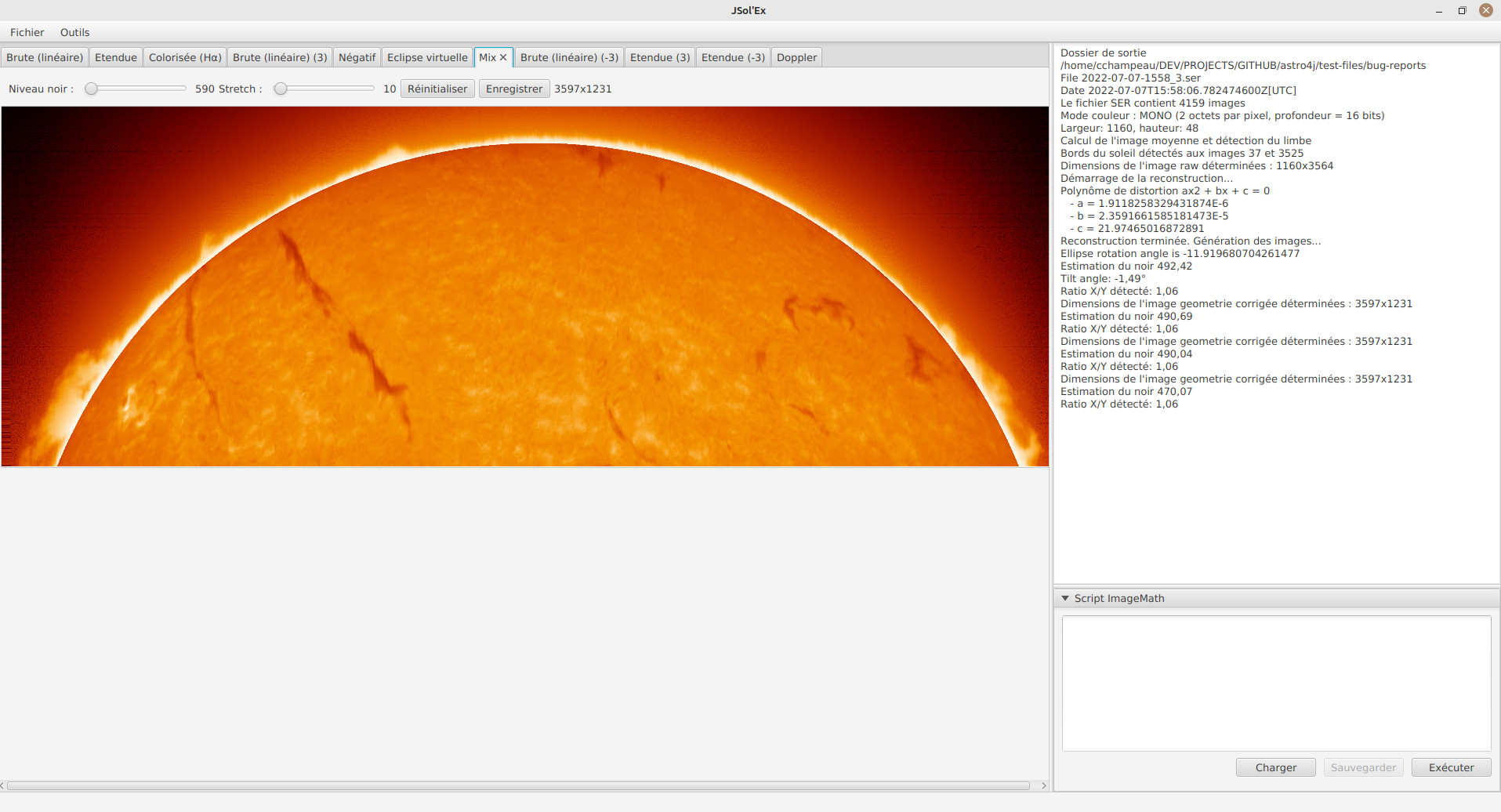
Processing a video file
JSol’Ex only supports SER files, please make sure to configure your capture software to use this format. The main window looks like this:
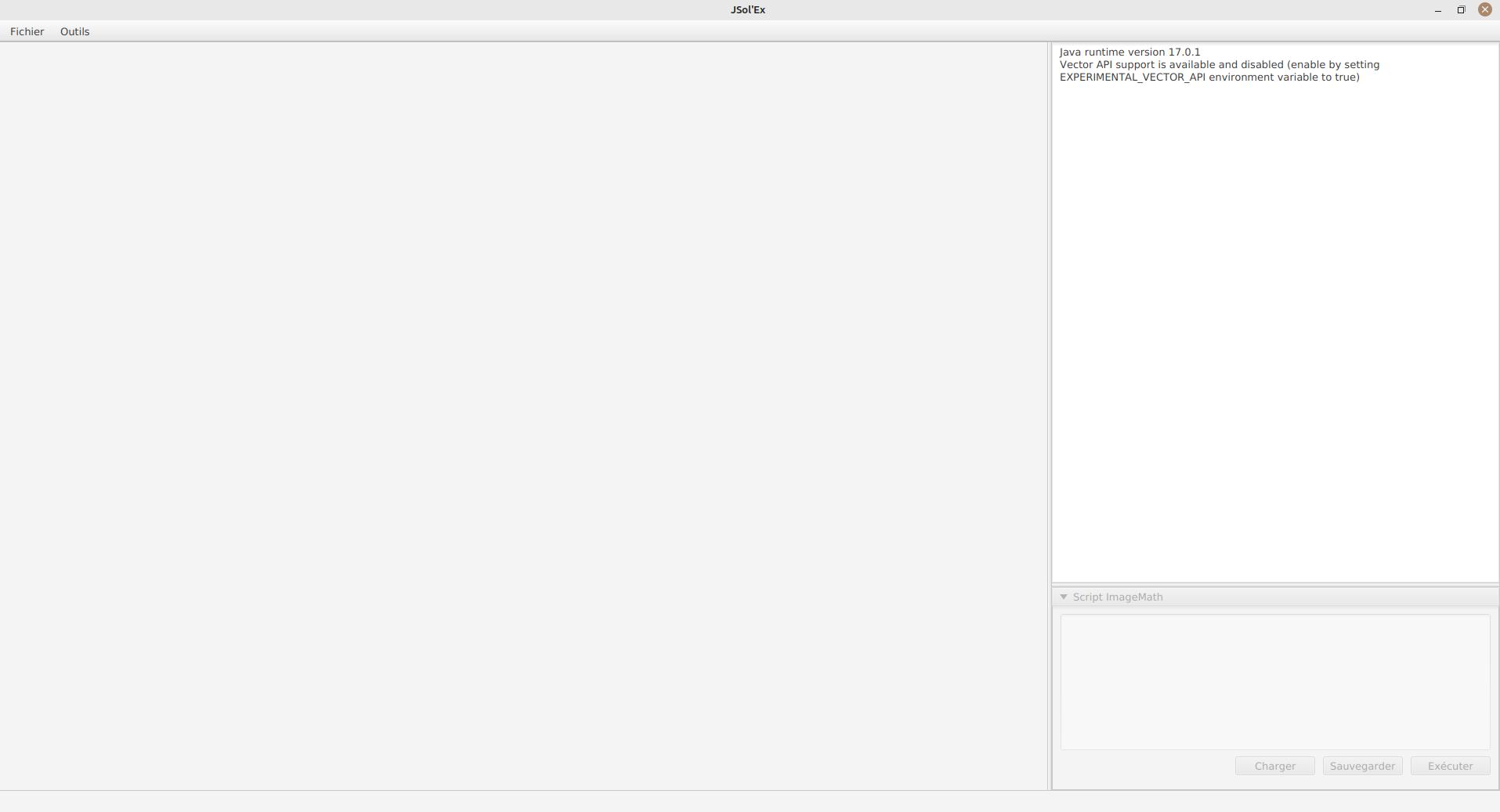
In the "File" menu, choose "Open SER File" and select a file. A configuration window opens, with several sections:
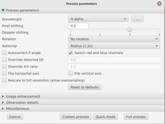
Basic parameters
The first section is the most important for your first scans, the other sections will help you refine the processing.
-
the observation bandwidth: while it’s not mandatory to select that field, doing so will enable automatic colorization of the images and advanced functionalities such as velocity calculations. By clicking on the "…" you have the possibility to add your own lines if they are not listed. This is the wavelength of the darkest line in your capture window. The "Autodetect" mode will try to find the line among those listed automatically.
-
Pixel shift : by default, the software will identify the darkest line in the image and model it as a second order polynomial. Then the image is reconstructed by picking the center of the line, which corresponds to a shift of 0. By using a different shift value, you can produce an image which is "off center", for example to produce images of the solar continuum or to select a different wavelength which isn’t the darkest, such as when observing in helium for example
-
the Doppler shift is only used when you are observing in h-alpha line to generate a Doppler image. By default, the software uses 2 images shifted by 3 pixels to reconstruct a color image.
-
the continuum shift is used to generate a continuum image, close to white light in H-alpha.
-
Red/blue channel inversion: when a Doppler image is created, the software assigns a shift to the red channel and the other to the blue channel. However, depending on your configuration, it may result in an image where the colors are inverted (regions approaching in blue instead of red). If this is the case, check this box to invert the channels.
-
Rotation : allows performing a left or right rotation (90 degrees) of the images. This can be useful for scans performed in declination, to fix the orientation. This parameter doesn’t affect images produced with ImageMath.
-
Autocrop : allows automatic cropping of images after geometric transformation. There are multiple modes:
-
Off: no autocrop (this is the default)
-
Original width: the image will be cropped to a square which width corresponds to the width of the original SER file. Ideal for full solar disks.
-
Radius (x…) : the image will be cropped or rescaled to a factor of the determined solar radius. This can be useful for example with truncated disks, if you want to "see" where it would be positioned.
-
-
Autocorrect P angle: when checked, the solar angle P will be computed from the observation date (available in the SER file). The generated images will be automatically corrected so that the North is at the top. This parameter will not affect images generated via ImageMath, which need to perform their own correction.
-
Horizontal and vertical inversion let you mirror the image so that you match the North and East as expected in the output images.
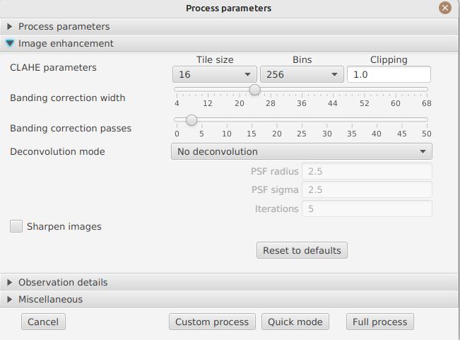
Cosmetic correction parameters
The second parameter panel allows you to configure cosmetic options:
-
Contrast enhancement method: you can choose between Autostretch (JSol’Ex), CLAHE and CLAHE (multi-scale). Depending on your choice, additional parameters will be available.
For the Autostretch method, you can configure:
-
gamma: a higher gamma will give a darker image
-
background correction: a value close to 0 will strongly suppress the sky background, a value close to 1 will keep it as is
-
prominence amplification: if enabled, allows choosing an amplification factor. The higher the factor, the more visible the prominences will be, at the cost of stronger demarcation with the limb
For the CLAHE method, you can configure:
-
tile size
-
number of histogram levels
-
clipping factor
The CLAHE (multi-scale) method runs CLAHE several times at tile sizes derived automatically from the solar disk diameter and averages the results. This greatly reduces the bright "ring" artifact that classic CLAHE can produce at the limb, while still enhancing local contrast at multiple scales. Only the clipping factor is configurable; tile sizes and histogram levels are chosen automatically.
Next come the banding correction parameters, which allow to correct transversal bands which can appear on images, for example because of dust on the slit.
-
Banding correction width: this is the width of the bands which are used in the transversallium correction algorithm. Bands are used to compute the average brightness of pixels in the band, then lines are corrected according the band they belong to.
-
Banding correction passes: the more passes you’ll apply, the more lines should be corrected, at the cost of lower contrast images
You can then choose detail enhancement parameters. By default, no deconvolution is applied, but you can choose the deconvolution algorithm and its parameters.
For the Richardson-Lucy deconvolution, you can choose the size of the synthetic PSF, the sigma factor and the number of iterations.
Finally, you can choose to apply a detail enhancement filter at the end of the processing. JSol’Ex provides three sharpening options:
-
None: No sharpening is applied
-
Sharpen: Traditional sharpening using a convolution kernel. You can adjust the kernel size (must be an odd number ≥ 3)
-
Unsharp Mask: More sophisticated enhancement technique that creates a mask from the difference between the original and a blurred version of the image. This method typically produces more natural-looking results with better edge preservation. You can adjust both the kernel size and the strength of the effect
Flat correction can be applied to images, in order to correct for vignetting or other artifacts. There are 3 modes available: - No correction: no correction is applied (this is the default) - Artificial flat correction: the software will compute a model of the flat field from the image itself, by looking at the pixels which are between a low and a high percentile. The model is then used to correct the image. This can be used to correct for reasonable vignetting. - Physical flat correction: the software can use a flat field which is either a SER file containing a few frames, or a pre-computed flat field. This is the preferred method for strong vignetting.
Jagged Edges Correction
This is an experimental feature available since JSol’Ex 3.1.0. It enables the correction of jagged edges which can appear on images. These jagged edges are common on images captured with a spectroheliograph and come from different causes:
-
atmospheric turbulence
-
wind
-
a mount that is not perfectly balanced or that is resonating
Jagged edges correction can reduce these defects dramatically. It only requires a single parameter: a "sigma" value which lets you adjust the number of points taken into account in the correction model. A value of sigma close to 0 will be very restrictive and will only correct small defects, while a higher sigma value will correct larger defects, at the risk of distorting prominences, for example.
|
Jagged edges correction may have side effects, such as distortion of prominences. It is not a perfect correction of atmospheric turbulence: indeed, it cannot correct effects perpendicular to the scan direction for example. Finally, it will work better on "low frequency" turbulence, that is, slow movements of the atmosphere, and less well on rapid movements. In all cases, it is recommended to start without correction and verify the result in all cases. |
Mount Oscillations Correction
This is an experimental feature available since JSol’Ex 5.3.2. Some mounts exhibit a regular, periodic oscillation during the scan, which shows up as a sinusoidal wave pattern on the solar limb. While jagged edges correction can reduce this defect, it corrects each line independently, which makes it sensitive to noise and can introduce artifacts.
The mount oscillations correction instead performs a spectral analysis of the limb position to find the dominant oscillation frequencies, then fits a model of the displacement and applies it to the whole image. The model is a sinusoid when the oscillation is stable, or a smoothed displacement curve when its period or amplitude drifts during the scan. Because the correction is driven by a global model rather than per-line measurements, it is insensitive to per-line detection noise, and it can also correct lines where the limb cannot be measured reliably, for example near the poles or outside of the disk.
If no significant periodic oscillation is detected, no correction is applied. The detected amplitude and period are written to the log, which can help diagnosing the mount. When debug images are enabled, a graph is also generated, showing the measured limb shift, the fitted oscillation model and the residual shift after correction. Both corrections can be enabled together: in this case the oscillation is removed first, and the jagged edges correction only deals with the remaining random defects.
Observation details
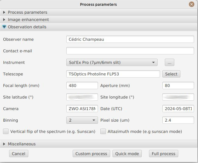
Observation parameters are used when you save your images in FITS format, to populate certain metadata. They are also used to calculate the wavelength graph.
Here are the fields available in JSol’Ex:
-
Observer : the person who made the observation
-
Email : the email address of the person who made the observation
-
Instrument : pre-filled to "Sol’Ex"
-
Telescope : your telescope or refractor used with the Sol’Ex instrument
-
Focal length and aperture of the telescope
-
Latitude and longitude of the observation site
-
Camera
-
Date : pre-filled with information from the SER file, expressed in the UTC timezone
-
Binning : the binning of pixels when the video was recorded
-
Pixel size : the size of the camera pixels in microns
-
Vertical flip of the spectrum : normally, the spectrum should have the blue wing at the top and the red wing at the bottom. If it’s the opposite, you can check this box. This is typically the case if you are using a Sunscan.
-
Alt-Az mode : check this box if you are not using an equatorial mount but an alt-az mount and that you are seeing an incorrect orientation of the image.
|
Alt-Az mode and image orientation correctness
It is important to understand that JSol’Ex is not capable of determining if an image is flipped vertically or horizontally, but it can compute the solar angle P from the observation date. However, the orientation grid that is generated will only be correct if you are using an equatorial mount. If you are using an alt-az mount, then the orientation grid will be incorrect, as well as the position of the labels of detected active regions. In order to fix this, you must check the "Alt-Az" box and enter your observation site coordinates: JSol’Ex will then compute the parallactic angle and perform correction automatically, resulting in a well oriented image. |
Images to generate
The following panel allows you to choose which images to generate.
In this section you can individually choose the images that interest you, or choose a predefined processing mode (quick or complete).
You can also choose to add ImageMath scripts to generate custom images (see the section on ImageMath).
-
Generate debug images: allows generating images such as edge recognition, ellipse/tilt recognition, average image. Useful to verify if the software is not behaving correctly on your video and you want to check where it goes wrong
Advanced processing parameters
These parameters are intended for special cases, to correct detection problems or for advanced work.
-
Force tilt value: during image geometric correction, JSol’Ex calculates an ellipse to model the reconstructed solar disk. This ellipse is used to calculate parameters like the tilt angle. If the calculation performed by the software is incorrect, you have the possibility to override the calculated value.
-
Force X/Y ratio: similarly, on certain images in difficult lines, the ellipse may not perfectly correspond to the solar disk and not reconstruct a perfectly circular sun. You can override the detected ratio to correct these problems
-
Force polynomial: allows forcing the second-degree polynomial used to model the spectral line. See the section on forcing the polynomial for more information.
-
Resize to maximum: can be used if your video is over-sampled and you want to keep the maximum resolution. This happens for example if you do scans at low speed (e.g., sidereal).
| Enabling this parameter can produce significantly larger images and cause high memory pressure. It is not recommended to enable this parameter. |
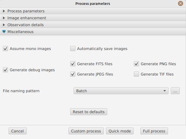
-
Assume mono video: when checked, JSol’Ex will not try to perform demosaicing of the video, by assuming it’s a mono one. This can considerably speedup processing, and because most videos for Sol’Ex will be mono, it is better to leave this checked.
Output parameters
In this section you can configure the file formats to generate as well as the file naming template.
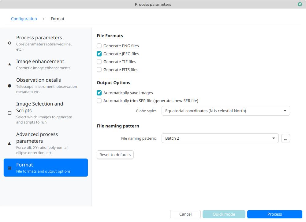
-
Automatically save images: if this box is checked, all generated images are automatically saved to disk. Otherwise, you will have to press the "Save" button in the interface that displays the generated images to keep the produced images
-
Generate FITS files: allows generating FITS files, non-destructive, in addition to PNG images
Force polynomial
JSol’Ex performs detection of the spectral line by looking for the darkest line in the image, then fitting a 3rd order polynomial to it. Sometimes, detection may be incorrect, in which case you can force a polynomial to be used.
In order to do this, click on the "force polynomial" button, which will let you enter the polynomial coefficients.
The format of the polynomial is a list of 4 numbers between curly braces, separated by commas, for example: {1.3414109042116584E-10,3.889927699830093E-5,-0.056529799336687114,35.76051527062038}.
The easiest way to get the polynomial coefficients is to click on the "…" button, which will open a window with the average image and the detected spectral line.
You can then press "CTRL" then click on the line to add measurement points: a red cross will be added for each point. When you have enough points, click on the "Compute polynomial" button, which will fit a 3rd order polynomial to the points and automatically fill the "polynomial" field in the process parameters.
Saturated disk mode
When the solar disk is overexposed (saturated), the spectral line can no longer be distinguished reliably, so JSol’Ex cannot detect the distortion polynomial from the scan itself. In this situation, you can capture one or more non saturated reference scans and let JSol’Ex reuse their polynomial.
Check the "Saturated disk mode" box (below "Force polynomial") and select the directory containing your non saturated reference scans. When processing a file, JSol’Ex looks up the reference scan which is the closest in time (based on the SER file dates) and applies its polynomial.
This mode is especially useful in batch processing: several saturated scans may share the same reference scan, in which case the reference polynomial is computed only once and reused.
If the closest reference scan is far away in time, a warning is issued because the polynomial may no longer be accurate. If no usable reference scan is found, JSol’Ex falls back to the regular automatic detection.
| "Saturated disk mode" and "Force polynomial" are mutually exclusive. |
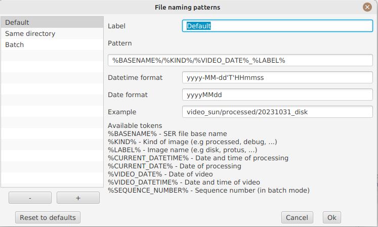
File naming patterns
By default, JSol’Ex will output the generated images in a subfolder which name matches the name of the SER file (without extension). Then each kind of images is stored in a subdirectory of that folder (e.g raw, debug, processed, …). If that naming convention doesn’t suit you, you can create your own naming patterns, by clicking the "…" dots:
A naming pattern consists of a label, but more importantly a pattern consisting of tokens delimited by the % character.
Please find below the list of available tokens:
-
%BASENAME%is the SER file base name, that is to say the name without extension -
%KIND%is the kind of images (raw, debug, processed, …) -
%LABEL%is the label of the produced images, e.grecon,protus -
%CURRENT_DATETIME%is the date and time of processing -
%CURRENT_DATE%is the date of processing -
%VIDEO_DATETIME%is the date and time of the video -
%VIDEO_DATE%is the date of the video -
%SEQUENCE_NUMBER%is the sequence number in case of batch processing (4 digits, eg.0012)
This for example would be a pattern which puts all generated files in a single folder:
%BASENAME%/%SEQUENCE_NUMBER%_%LABEL%
The "example" field shows you what the generated file names would look like.
User-Defined Presets
In addition to the built-in "Quick Mode" and "Full Process" presets, JSol’Ex allows you to create and manage your own custom presets for image selection and script configuration.
Creating a Preset
Once you have configured your desired image selections and scripts in the "Custom Images and Scripts" section, you can save your configuration as a preset:
-
Select the images you want to include in your preset
-
Configure any ImageMath scripts if needed
-
In the "Custom Images and Scripts" section, click the "Save as Preset…" button
-
Enter a descriptive name for your preset
-
Click "OK" to save
Your preset is now saved and will persist between JSol’Ex sessions.
Using Your Presets
User-defined presets appear as buttons in the processing parameters window, alongside the Quick Mode and Full Process buttons. Simply click on any preset button to instantly apply that configuration.
Each preset restores: - All image type selections (basic, advanced, and custom images) - ImageMath script configurations - Automatic scripts setting
Managing Presets
-
Load a preset: Click on the preset button to apply its configuration
-
Delete a preset: Click the "×" button next to any user preset to remove it (with confirmation)
-
Replace a preset: Save a new preset with the same name as an existing one to replace it
User presets are stored locally on your computer and are automatically available every time you open JSol’Ex.
Starting a process
When you have configured the parameters, click "Process" to start the processing.
You have the possibility to launch a quick or complete processing directly by clicking the corresponding buttons in the bottom right.
Image display
Once images are generated, they appear one after each other in tabs. These tabs provide you with the ability to tweak the contrast of images and save them, typically when you unchecked the automatic save option.
It is possible to zoom into the images by using the mouse wheel. In addition, right-clicking the image will let you open it into your file explorer or in a separate window.
You can also duplicate an image from the sidebar by right-clicking on its name and choosing "Duplicate", which is useful when you want to keep a clean original alongside an annotated version.
Other spectral lines in the capture window
The captured window often contains known spectral lines other than the one you are studying. For example, when imaging in Calcium H, the H-epsilon line usually falls within the same window.
When this happens, JSol’Ex marks each of these lines with a dotted vertical marker, labelled with the line name, on the spectral profile graph, and automatically reconstructs a dedicated image at that line’s position, exactly as if you had added its pixel shift manually.
Annotations
Each image has its own set of annotations that you can turn on or off independently from the annotations panel, opened with the ⊕ button in the toolbar. The panel is a floating popover that you can drag around the screen while you work.
The following annotations are available:
-
Colorize: applies a color to a monochrome image, which is useful as a backdrop for colored annotations. This option only appears for monochrome images. From its options menu you can pick a spectral profile (e.g. H-alpha, Calcium, Helium) or a custom color; the default profile matches the spectral line of the image. A "Preserve brightness" option keeps the original luminance so colorizing only adds hue without darkening the image. RGB images are left untouched.
-
Orientation grid: heliographic meridians and parallels drawn on the solar disk, with the rotation axis and cardinal direction markers. The grid style (equatorial or solar coordinates) and the P-angle correction can be tweaked from the grid options menu.
-
Prominence scale: dashed concentric circles outside the solar limb with distance labels in kilometres. You can choose the number of circles and the spacing between them.
-
Active regions: the NOAA active region numbers placed at their position on the solar disk. From the options menu you can optionally draw a rectangle around each region, and set the P-angle correction for ImageMath images.
-
Observation details: a block of text usually placed in the top-left corner with the observer name, date, instrument, telescope, camera, etc. The content is fully editable through a template with placeholders (e.g.
%OBSERVER%,%DATETIME%,%TELESCOPE%), so you can pick exactly which fields are shown, reorder them, or add your own text. Empty lines (where the value is missing) are skipped automatically. -
Solar parameters: a block listing the P, B0 and L0 angles together with the Carrington rotation, placed in the top-right corner.
-
Earth size reference: a small Earth picture overlaid on the image as a size comparison. The marker is draggable: click and hold to move it where you want.
-
Signature: free text rendered in the bottom-left corner. You can pick the font (the dropdown previews each typeface in its own style), the size and the weight.
-
Text areas: an arbitrary number of free-text annotations that you place anywhere on the image by dragging them. Use the "Add text area" button at the bottom of the panel to create one; each has its own text, font, size, weight and color, and can be removed with its trash button.
Each annotation has its own color, with the default being a neutral gray that preserves monochrome images. A global line thickness control at the bottom of the panel lets you make all drawn lines bolder or thinner.
When editing the signature or the observation details template, the changes preview live on the image. Click "Apply" to keep them or "Close" to revert.
You can save the current annotation settings (toggles, colors, line thickness, prominence scale options, observation details template, signature) as a preset with the "Save preset" button at the bottom of the panel, and reload them on any other image with "Load preset". The preset is stored on your computer and persists across JSol’Ex sessions.
Exporting and importing sessions
After processing one or more files, you often want to compare the results and later share the best image, for example on SpectroSolHub. Instead of reprocessing the original SER video, you can export the current state of the image viewer to a session file and reopen it whenever you need it.
To export, choose "Export session…" from the File menu and pick a destination.
The session file (.jsxs) stores every generated image, the animations and videos, and their processing parameters.
The file is compressed, but keep in mind that a session containing many images can still be large.
To restore a session, choose "Import session…" from the File menu and select a .jsxs file.
If the viewer already contains images, JSol’Ex asks whether you want to replace them or merge the imported ones with the current view.
The restored images keep their original parameters, so you can save, annotate or share them exactly as if they had just been processed, without touching the original video.
Watching a directory for changes
When trying to find the ideal focus, it can be useful to process video files quickly until we obtain a satisfying result. JSol’Ex offers an easy way to do this, by watching the changes in a directory : new videos which are saved in that directory will immediately be processed.
To do this, in the file menu, choose "Watch directory" then select the directory where your SER files will be recorded (e.g the output directory of SharpCap).
JSol’Ex will switch to watch mode, which you can interrupt by clicking the button which appeared in the bottom left of the interface.
Now, open your capture software and record a new video. Once it’s done, switch to JSol’Ex : it will open the process parameters configuration window. Select your processing parameters then start the processing.
Once you have the result, switch back to your capture software and acquire a new video. Once its done, switch back to JSol’Ex: this time, the process parameters window won’t open, because it’s going to reuse the parameters from the first video, allowing to process new videos very quickly!
| Make sure that when you switch from your capture software to JSol’Ex that the recording is finished. If not, processing can start on an incomplete file and fail. |
Once you’re happy with the result, click on the "Stop watching" button on the bottom left.
| You can combine the watch mode with opening an image in a new window (by right-clicking on an image, you can open it in a new window). When a new SER file will be processed, the corresponding image will automatically replace the one in the external window. This can be useful in demonstrations, if you have for example a separate monitor where you would only show the result of processing. |
Importing scans from a SunScan
If you own a SunScan spectroheliograph, JSol’Ex can fetch the scans acquired by the device directly, without having to copy files manually.
Connect your computer to the SunScan Wi-Fi access point, then in the "File" menu choose "Import from SunScan…".
JSol’Ex will try to locate the device automatically on the network. If detection fails, type its address (for example sunscan.local:8000) in the "Device address" field and click "Connect".
The dialog lists every scan available on the device, with its acquisition date, spectral line and processing status. Tick the scans you want to process, choose a download folder, then click "Import and process". JSol’Ex downloads the selected scan.ser files (renamed YYYY_MM_DD-HH_mm_ss-scan.ser based on each scan’s UTC capture date) and opens them: a single scan opens the regular processing window, while several scans are processed as a batch.
When scans are imported this way, the "Sunscan" instrument and its setup (camera and pixel size) are selected automatically in the processing parameters, which also enables the vertical flip of the spectrum. You can still change these settings before starting the processing.
Customization of generated images
When you click the "custom" mode instead of the quick or full ones, JSol’Ex provides you with an interface which will let you declare exactly what should be output.
There are 2 modes available: the simple one and the ImageMath one.
In the simple one, you can pick which images to generate by clicking the right boxes. It is also possible to ask for the creation, in parallel, of images at different pixel shifts.
For example, should you want to generate images from the continuum to the observed ray, you can enter -10;-9;-8;-7;-6;-5;-4;-3;-2;-1;0;1;2;3;4;5;6;7;8;9;10 which will have the consequence of generating 21 distinct images ranging from shift -10 to +10.
This can be particularly useful if you want, for example, to generate an animation.
It’s worth noting that if you check some images like "Doppler", some pixel shifts will be automatically added to the list (e.g -3 and +3).
If this isn’t good enough for you, you can go even more advanced by enabling the "ImageMath" mode which is extremely powerful while relatively simple to grasp.
Trimming SER files
It is not unsual to have SER files which contain a lot of empty frames at the beginning or at the end, because of how we usually capture videos: we start the capture, then we wait for the mount to stabilize, then we stop the capture. In addition, our cropping window may be a bit too large for what we actually want to study.
As a consequence, SER files stored on disk are usually significantly larger than what they need to be. Since JSol’Ex 2.10, a new option is available at the end of the processing of a file. You can click on the "Trim SER file" button on the top right corner of the interface, which will open a new window:
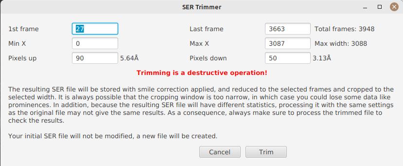
This window is pre-filled with parameters which are deduced from the processed file. In particular, the start and end frames, as well as the mininum and maximum X values (width) are automatically determined from the detection of the solar disk in the video. A reasonable margin of 10% is added, which means that sometimes, the first and last frame may actually correspond to the full video if you actually have video where the sun appears quickly in the field of view.
The "pixels up" and "pixels down" parameters correspond to how many pixels you want to keep in the target SER file. Again these are automatically determined from the correction of the "smile" (the curvature of the spectral line), but it may be particularly interesting to reduce, since it will have a large impact on the size of the file. However, reducing the number of pixels up/down will remove information from the video (you won’t be able to compute images with larger pixel shifts), so always be careful not to reduce it too much.
Once you’re happy with the parameters, click on "Trim" and a new SER file will be created in the same directory as the original one, with the suffix _trimmed.
It’s worth noting that the trimmed video will also have the smile correction applied, which means that the spectral line will be centered in the video and that each line will be perfectly horizontal. This information is used by JSol’Ex in case you decide to process the trimmed video, so that you don’t have to recompute the smile correction.
|
It is important to understand that trimming is a destrutive operation: when you reduce the number of frames or the min x/max x values, then you are potentially truncating the solar disk or features like prominences. If you are selecting too low pixel up/down values, then you are reducing the bandwidth of observation, which means for example that you may not be able to generate a continuum image anymore. In both cases, the result of processing the trimmed video will be different from the original one. |
Here’s an example of a video:
And the result after trimming:
Creating Image Collages
JSol’Ex includes a collage feature that allows you to combine multiple processed images into a single composite image. This is useful for creating comparison views or presentation materials.
Accessing the Collage Feature
The collage feature becomes available after processing images. Once you have at least two non-reconstruction images available:
-
Look for the "Actions" section in the left sidebar
-
Click on "Create collage" link
Using the Collage Interface
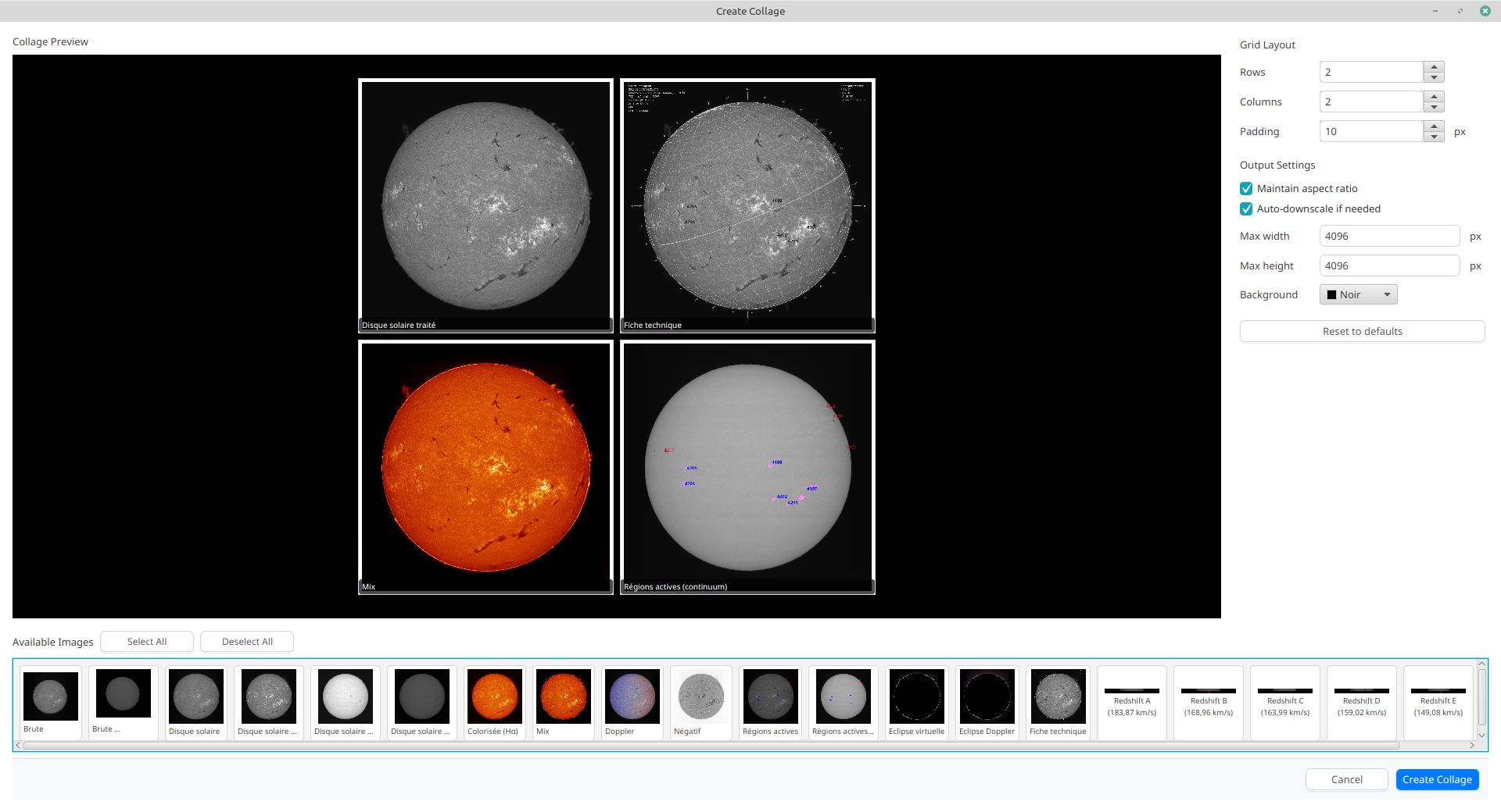
The collage interface provides a drag-and-drop workspace where you can:
-
Select Grid Layout: Choose the number of rows and columns for your collage
-
Add Images: Drag images from the image strip at the top to empty slots in the grid
-
Rearrange Images: Drag images between slots to reorder them
-
Remove Images: Double-click on a slot to remove an image
-
Customize Appearance: Adjust spacing between images and set the background color
Collage Controls
-
Rows/Columns: Define the grid dimensions (1-10 rows/columns)
-
Spacing: Set the pixel gap between images (0-50 pixels)
-
Background Color: Choose the color for empty areas and spacing
-
Max Width/Height: Set maximum output dimensions (images will be scaled proportionally if needed)
Creating the Collage
Once you have arranged your images:
-
Click the "Create" button to generate the collage
-
The collage will be saved to your output directory
-
The new collage image will appear in the main image viewer
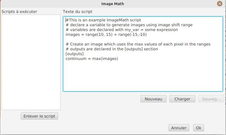
ImageMath : images generation scripts
Introduction to ImageMath
The "ImageMath" mode is a mode which will let you declare which images to generate by writing small scripts. It relies on a simple script language designed specifically for generating Sol’Ex images.
Let’s illustrate this by going back to our previous example, where you wanted to generate images in the [-10;10] pixel shift range. In the "simple" mode, you had to manually enter all pixel shifts, which can be a little cumbersome. In the "ImageMath" mode, we have a language which will let us to this with a single instruction.
First, select the ImageMath mode in the select box and click on "Open ImageMath".
The following interface show up:
On the left side, "Scripts to execute", you will find the list of all scripts which will be applied in your session.
| This is really the list of scripts which are applied in that session, not the list of available scripts! Click on the "remove" button to remove scripts from execution in the session. |
Scripts must be saved on your local disk and can be shared with other users. Their contents is editable in the rightmost part of the interface.
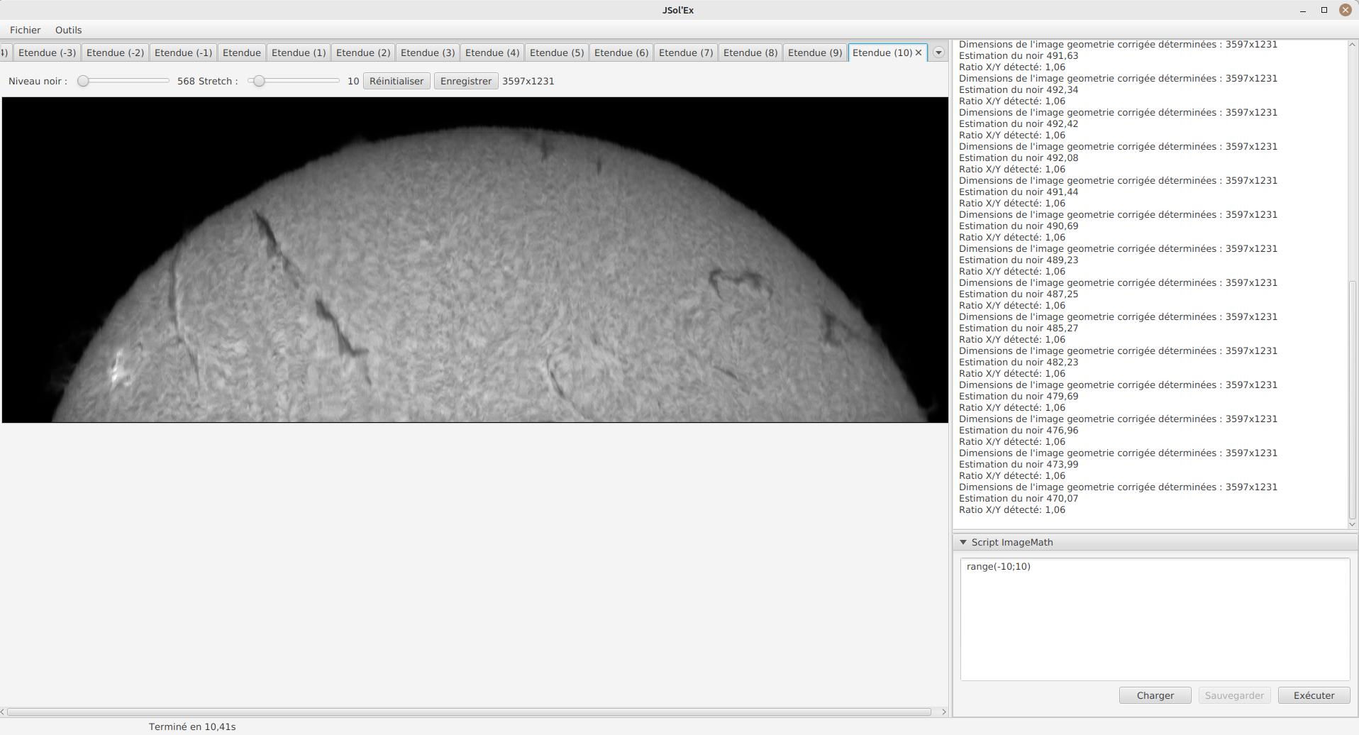
Start with removing the contents of the sample script and replace it with:
range(-10;10)Then click on "Save". Select a destination file and proceed: the script is now added to the list on the left, as being executed in this session.
Click on "Ok" to close ImageMath and only keep the "geometry corrected (stretched)" images. Click on "Ok" to start processing, you will now have the 21 required images generated:
Functions available in ImageMath
For now we’ve only used one function called range, which let us generate about 20 images, but there are many others available.
Please refer to this page for the complete list of functions available in ImageMath.
ImageMath scripts
In the previous section, we have seen the building blocks of ImageMath, which permit computation of new images. Scripts go beyond this by combining these into a powerful tool to generate images. As an illustration, let’s look at this script which will let us generate an Helium image. Helium image processing is complicated, because the Helium ray is very dim and the software cannot find it in the image. Therefore, we can use a technique which consists of taking a larger capture window which includes a dark ray, then by determining by how many pixels the helium ray is shifted from that line, we can reconstruct an image. Even so, the work is not finished, since it’s an extremely low contrast ray, so we have to substract the continuum value. Producing such images is quite cumbersome but can be simplified to the extreme with ImageMath:
[params]
# The shifting between the helium line and the detected line (in pixels)
Line=5875.62
HeliumShift=find_shift(Line)
# Banding correction width and number of iterations
BandWidth=25
BandIterations=20
# Contrast adjustment
Gamma=1.5
# Autocrop factor (of diameter)
AutoCropFactor=1.1

## Temporary variables
[tmp]
helium_raw = img(HeliumShift) - continuum()
helium_fixed = fix_banding(helium_raw;BandWidth;BandIterations)
cropped = autocrop2(auto_contrast(helium_fixed;Gamma);AutoCropFactor)

## Let's produce the images now!
[outputs]
helium_mono = cropped
helium_color = colorize(helium_mono, Line)
Our script consists of 3 different sections: [params], [tmp] and [outputs].
The only mandatory section is the [outputs] one: it defines which images we want to have in the end.
The name of all other sections is arbitrary, you can create as many sections as you want.
Here, we defined a [params] section which highlights which parameters we want users to be able to tweak for their needs.
This is where we find the value of our helium ray pixel shift (HeliumShift=find_line(Line)) which is computed from the Line=5875.62 variable declaration.
A variable can only contain ASCII characters, digits (except for the 1st character) or the _ character. For example, myVariable, MyVariable or MyVariable0 all all valid identifiers. hélium is invalid (because of the accent).
|
Variables can be used in other variables or function calls.
Variables are case sensitive. myVariable et MyVariable are 2 distinct variables!
|
Our 2d section, [tmp], defines intermediate images we want to work with, but for which we don’t care about seeing the result:
-
helium_rawis the Helium ray image, shifted from the detected ray and from which we have subtracted the continuum image. -
helium_fixedis thehelium_rawimage to which we have applied the banding correction algorithm. -
croppedis thehelium_fixedimage to which we have applied an autocrop and a contrast adjustment.
Last but not least, the [outputs] section declares the images we want to generate:
-
helium_monois thecroppedimage as is, in black and white. -
helium_coloris thehelium_monoimage to which we have applied a colorization.
Comments can be added either with the # or // prefix.
|
Script Parameters
Scripts can optionally declare configurable parameters using the meta block.
While not required, adding parameters is highly recommended if you plan to share your script with others, as users unfamiliar with scripting will prefer tweaking parameters rather than modifying code directly.
When a script declares parameters, JSol’Ex automatically creates user interface controls that allow users to adjust values without editing the script.
Declaring Parameters
Parameters are declared in a meta block at the beginning of your script:
meta {
    title = "Enhanced Stacking Script"
    requires = "4.1.0"

    params {
        tileSize {
            type = "number"
            default = 64
            min = 16
            max = 512
            name {
                en = "Tile Size"
                fr = "Taille de tuile"
            }
            description {
                en = "Size of tiles for processing"
                fr = "Taille des tuiles pour le traitement"
            }
        }

        pixelShift {
            type = "number"
            default = 0
            min = -10
            max = 10
            name = "Pixel Shift"
            description = "Shift in pixels from reference wavelength"
        }

        cropRatio {
            type = "choice"
            choices = "1.0,1.1,1.2,1.5,2.0"
            default = "1.1"
            name = "Autocrop Ratio"
            description = "Solar radius multiplication factor for cropping"
        }
    }
}

[outputs]
result = autocrop(img(pixelShift), cropRatio)
Parameter Types
JSol’Ex supports three parameter types:
-
number: Numeric values with optional min/max constraints
-
string: Text values
-
choice: Selection from predefined options
Meta Block Properties
-
title: Display name for the script (supports multiple languages)
-
requires: Minimum JSol’Ex version needed (displays warning if not met)
-
params: Container for parameter definitions
-
requirements: Container for declaring image kinds that must be generated for the script to work (see Script Requirements)
Script Requirements
A script may declare image kinds that it needs to perform its job. When a script is executed, any GeneratedImageKind listed in the requirements block will be added to the list of images to generate, as if the user had explicitly selected them in the image selection panel.
meta {
    title = "Active regions on continuum"
    requirements {
        images = [ "CONTINUUM", "ACTIVE_REGIONS" ]
    }
}
Unknown image kinds are silently ignored. Implied kinds are automatically included (for example ELLERMAN_BOMBS implies FLARES).
Localization
Parameter names and descriptions can be localized using language objects or simple strings:
name {
    en = "English Name"
    fr = "Nom français"
}
// Or simply:
name = "Default Name"
If no localization is provided for the user’s language, JSol’Ex falls back to English, then to the first available language.
Version Compatibility
The requires field ensures users are warned if their JSol’Ex version might not support all script features:
meta {
    requires = "4.1.0"  // Warns users with older versions
}
Special variables
This table summarizes the special variables which are exposed to ImageMath scripts:
| Variable | Description |
|---|---|
|
The computed black point of the image |
|
The computed solar P angle (in radians) |
|
The computed B0 angle (in radians) |
|
The computed L0 angle (in radians) |
|
The Carrington rotation number |
|
The detected wavelength of the image (in Angström), corresponding to the image |
Custom functions
In addition to the functions provided by JSol’Ex, it is possible to define your own functions, which combine existing functions. For example, let’s say that you would like to draw the globe, technical details and solar parameters on more than one image. You script may look like this:
image1=draw_obs_details(draw_solar_params(draw_globe(img(0))))
image2=draw_obs_details(draw_solar_params(draw_globe(auto_contrast(img(0);1.5))))
Instead of repeating the same function calls on several images, we can declare a function which would do this for us:
[fun:decorate img]                                              (1)
   result=draw_obs_details(draw_solar_params(draw_globe(img)))  (2)

[outputs]
image1=decorate(img(0))                                         (3)
image2=decorate(auto_contrast(img(0);1.5)) (4)| 1 | The function declaration. The name of the function is decorate, and it takes a single argument, img. |
| 2 | The function must end with an assignment to the result variable. |
| 3 | The function is then called with the img(0) image. |
| 4 | The function can also be called with the auto_contrast(img(0);1.5) image. |
Functions must be declared at the beginning of the script.
They can take any number of arguments, but they must always return a value in the result variable.
If you declare a function, you must have a section which separates the functions declarations from your main script (for the [outputs] section).
A function can consist of intermediate expressions and can call other functions. For example, let’s create a function which will display our image with a title:
[fun:titled img title]                                          (1)
   decorated=decorate(img)                                      (2)
   result=draw_text(decorated, 10, 10, title)

[fun:decorate img]
   result=draw_obs_details(draw_solar_params(draw_globe(img)))

[outputs]
image1=titled(img(0))                                         (3)
image2=titled(auto_contrast(img(0);1.5)) (4)| 1 | The titled function declaration. It takes 2 arguments: img and title. |
| 2 | The titled function calls the decorate function, then adds a title to the image. |
| 3 | The titled function is then called with the img(0) image. |
| 4 | The titled function can also be called with the auto_contrast(img(0);1.5) image. |
|
Passing a list to a function
The first argument of a function is always treated differently.
If it is passed a list, then the function will be called for each element of the list, then the results will be collected in a list.
For example, if we call the |
Including other scripts
It is possible to include other scripts in your script.
This can be useful if you have a set of functions which you want to reuse in several scripts.
For example, we could extract the function definitions from the previous example and put them in a separate file, functions.math:
[fun:decorate img]
   result=draw_obs_details(draw_solar_params(draw_globe(img)))
[fun:titled img title]
   decorated=decorate(img)
   result=draw_text(decorated, 10, 10, title)
Then it can be included in another script:
[include "functions"]

[outputs]
image1=titled(img(0), "My first image")
image2=titled(auto_contrast(img(0);1.5), "My second image")|
Includes are resolved relatively to the script which includes them. |
Remote script generation
|
This feature is experimental and may change in the future. It is designed for advanced users who are comfortable with programming. |
ImageMath is an expression language. It doesn’t support control structures like loops or conditionals, which can sometimes be limiting. In addition, sometimes you may want to perform operations which are not available in the language itself.
To support these advanced use cases, a special function named remote_scriptgen is available.
This function will call a service which will be responsible for generating a script which will contribute new variables to the current context.
The function accepts a single argument, which is a URL to the service.
JSol’Ex will then create a POST request to this URL, with a JSON payload which contains the current context, that is to say the list of variables with their values at the time of the call, but also context like the processing parameters or the detected wavelength.
The JSON payload consists of 2 top level keys:
{
  "variables": {
     ... one key per variable ...
  },
  "context": {
    ... the process parameters ...
  }
}
The variables can be simple values, like numbers or strings, but also arrays or objects like images:
{
  "variables": {
    "detectedWavelen": 6562.8099999999995,
    "detectedDispersion": 0.10878780004221283,
    "l0": "4.4165",
    "src": {
      "type": "image",
      "width": 1424,
      "height": 1424,
      "file": "/tmp/jsolex/1960308/image9339121918435728514.fits",
      "metadata": {
        "sourceInfo": {
          "serFileName": "12_08_34.ser",
          "parentDirName": "christian",
          "dateTime": "2021-09-05T10:08:34.806652200Z[UTC]"
        },
        "pixelShiftRange": {
          "minPixelShift": -20.0,
          "maxPixelShift": 40.0,
          "step": 6.0
        },
        "solarParameters": {
          "carringtonRotation": 2248,
          "b0": 0.12636308214692193,
          "l0": 4.416504789595021,
          "p": 0.38650968395297775,
          "apparentSize": 0.0091870061684479
        },
        "pixelShift": {
          "pixelShift": 0.0
        },
        "transformationHistory": {
          "transforms": [
            "Rotate left",
            "Flipping",
            "Banding reduction (band size: 24 passes: 16)",
            "Geometry correction",
            "Autocrop",
            "ImageMath: img(0)",
            "ImageMath: img(0)",
            "ImageMath: img(0)",
            "ImageMath: src\u003dimg(0)",
            "ImageMath: range(-1;1;.5)",
            "ImageMath: range(-1;1;.5)",
            "ImageMath: range(-1;1;.5)",
            "ImageMath: range(-1;1;.5)",
            "ImageMath: img(0)",
            "ImageMath: img(0)",
            "ImageMath: img(0)",
            "ImageMath: src\u003dimg(0)"
          ]
        },
        "ellipse": {
          "a": 0.7071067811865355,
          "b": -1.1224941413357953E-13,
          "c": 0.7071067811865596,
          "d": -1006.9200564095466,
          "e": -1006.9200564095809,
          "f": 423490.4527558379
        },
        "generatedImageMetadata": {
          "kind": "IMAGE_MATH",
          "title": "src",
          "name": "batch/2025-03-26T225606/src/0000_12_08_34_src"
        }
      }
    },
    "blackPoint": "283.533",
    "angleP": "0.3865",
    "some_var": 123.0,
    "b0": "0.1264",
    "carrot": "2248"
  }
}
In case of an image, the object will have a key of type with value image.
The file will be available as a FITS file only.
|
The file path is the path to the FITS file, which is a temporary file, on the host which runs JSol’Ex.
Therefore, you will only be able to access this file from the same host!
This can also be used to generate new images, which can be loaded in JSol’Ex if the script that is returned contains a |
The service must return a JSON object which contains a script key, with the script to execute in JSol’Ex.
It can also return an object with an error key, which will be displayed to the user.
The scripts which are returned from the server are interpreted in a separate context, but they share the variables and user functions from the including script. The separation means that the script which is returned can itself be organized in sections, but only the outputs section will contribute new variables to the context.
For example, if a server returns the following script:
[tmp]
base=auto_contrast(img(0);1.5)

[outputs]
final=draw_obs_details(draw_solar_params(draw_globe(base)))
Then only the final variable will be visible to the including script after execution.
|
When a script calls the |
For advanced scripting capabilities, JSol’Ex also supports Python. Please refer to the Python scripting documentation for details.
Script Repositories
JSol’Ex supports script repositories, allowing you to discover and automatically download ImageMath scripts published by the community. Repository scripts appear alongside built-in scripts in the image selection panel and are automatically updated when new versions are published.
Using Script Repositories
Adding a Repository
To add a script repository:
-
Open the Tools menu and select "Script Repositories…"
-
Click the "Add" button
-
Enter a name for the repository (for display purposes)
-
Enter the repository URL (must start with
http://orhttps://) -
Click "Add"
JSol’Ex will immediately fetch the available scripts from the repository.
Managing Repositories
The Script Repositories dialog displays:
-
Name: The repository name you provided
-
URL: The repository address
-
Scripts: Number of scripts available
-
Last Check: When the repository was last checked for updates
You can:
-
Edit: Change the repository URL (the name cannot be changed)
-
Remove: Delete a repository and its cached scripts
-
Refresh: Manually check for new or updated scripts
Using Repository Scripts
Repository scripts appear in the image selection panel alongside built-in scripts. They are organized by repository name and display metadata including:
-
Script title
-
Author name
-
Version number
Select repository scripts the same way as built-in scripts. If a script declares parameters in its metadata block, you’ll be able to configure them in the UI.
Automatic Updates
JSol’Ex checks repositories for updates:
-
Once per day at startup
-
When you click the Refresh button in the Script Repositories dialog
Scripts are automatically updated when a newer version is detected based on the version field in the script metadata.
Version Compatibility
When checking for updates, JSol’Ex ensures version compatibility:
-
Scripts without a
requiresfield are always downloaded (assumed compatible with all versions) -
Scripts with
requiresset to a version newer than your current JSol’Ex version are ignored -
If you have a local compatible version of a script, it is preserved even if a newer incompatible version is published
Publishing Scripts
If you want to share your ImageMath scripts with the community, you can publish them via a script repository.
Repository Structure
A script repository is simply an HTTP server that exposes .math files.
JSol’Ex supports two discovery methods:
1. scripts.txt file (recommended)
Create a scripts.txt file listing available scripts (one filename per line):
# My repository
my-script.math
another-script.math
Comments start with # and are ignored.
2. Directory listing (fallback)
Enable directory listing on your web server (Apache mod_autoindex, nginx autoindex):
http://example.com/scripts/
  ├── my-script.math
  ├── another-script.math
  └── ...
JSol’Ex will try to download scripts.txt first, and fall back to parsing HTML directory listings if not found.
Zip File Support
For scripts that require additional files (such as Python modules), you can bundle them in a .zip archive.
JSol’Ex will automatically extract the contents when downloading from a repository.
Zip file structure:
my-script.zip
├── my-script.math       # Main script
├── main.txt             # Optional: specifies main script (required if multiple .math files)
├── utils.py             # Python modules
└── helpers.py
Rules for determining the main script:
-
If there is only one
.mathfile in the zip, it is automatically used as the main script -
If there are multiple
.mathfiles, you must include amain.txtfile containing the name of the main script
The directory structure inside the zip is preserved, so scripts can reference files using relative paths like python_file("utils.py").
Example main.txt:
my-script.mathList zip files in scripts.txt alongside regular .math files:
# My repository
simple-script.math
bundled-script.zip
Script Requirements
For a script to be available in a repository, it must:
-
Have a
.mathextension -
Include a metadata block with required fields
-
Be accessible via HTTP/HTTPS
Metadata Block Format
Each script must include a metadata block with at minimum:
-
author: Script author name -
title: Script title (displayed in UI, can be multilingual) -
version: Script version for update tracking
Optional fields include:
-
requires: Minimum JSol’Ex version required (e.g.,"4.2.0"). Users running older versions will not download scripts with incompatible version requirements. -
description: Script description (can be multilingual) -
params: Parameter declarations with types, defaults, and descriptions
Example with multilingual support and parameters:
meta {
    title {
        en = "My Processing Script"
        fr = "Mon script de traitement"
    }
    author = "John Doe"
    version = "1.0"
    requires = "4.2.0"
    params {
        gamma {
            type = "number"
            default = 1.5
            min = 0.1
            name {
                en = "Contrast Gamma"
                fr = "Gamma contraste"
            }
            description {
                en = "Gamma correction value"
                fr = "Valeur de correction gamma"
            }
        }
    }
}
The metadata block must appear at the beginning of the script file.
Version Updates
When you publish a new version of a script, update the version field in the metadata block.
It is recommended to use semantic versioning (e.g., 1.0, 1.1, 2.0).
Users will automatically receive the updated script the next time JSol’Ex checks for updates.
Example Repository
A minimal script repository might look like:
http://example.com/jsolex-scripts/
  ├── scripts.txt
  ├── stacking.math
  └── continuum-subtract.math
With scripts.txt:
# My JSol'Ex Scripts
stacking.math
continuum-subtract.math
And stacking.math with full metadata and parameters:
Click to expand full script example
meta {
    title {
        en = "Stacking"
        fr = "Empilement"
    }
    author = "Cédric Champeau"
    version = "1.0"
    requires = "4.2.0"
    params {
        method {
            type = "choice"
            choices = ["sharpness", "average", "median", "manual"]
            default = "average"
            name {
                en = "Best image selection method"
                fr = "Méthode de sélection de la meilleure image"
            }
            description {
                en = "Method used to select the best image as a reference for stacking"
                fr = "Méthode utilisée pour sélectionner la meilleure image comme référence pour l'empilement"
            }
        }
        gamma {
            type = "number"
            default = 1.5
            min = 0.1
            name {
                en = "Final Contrast Gamma"
                fr = "Gamma contraste final"
            }
            description {
                en = "Gamma correction value for the final contrast adjustment"
                fr = "Valeur de correction gamma pour l'ajustement final du contraste"
            }
        }
        tileSize {
            type = "number"
            default = 64
            min = 16
            name {
                en = "Tile Size"
                fr = "Taille des tuiles"
            }
            description {
                en = "Size of the tiles used for dedistortion. Must be a power of 2."
                fr = "Taille des tuiles utilisées pour les calculs de déformation. Doit être une puissance de 2."
            }
        }
        sampling {
            type = "number"
            default = 0.25
            min = 0.125
            max = 1.0
            name {
                en = "Sampling"
                fr = "Échantillonnage"
            }
            description {
                en = "Sampling factor for the local normalization and dedistortion (between 0.125 and 1.0)"
                fr = "Facteur d'échantillonnage pour la normalisation locale et la déformation (entre 0.125 et 1.0)"
            }
        }
        ratio {
            type = "number"
            default = 1.0
            min = 0.1
            name {
                en = "Proportion of images used for stacking"
                fr = "Proportion d'images utilisées pour l'empilement"
            }
            description {
                en = "Proportion of images to keep for stacking (1 means keep all images, 0 would keep none)"
                fr = "Proportion d'images à conserver pour l'empilement (1 signifie conserver toutes les images, 0 n'en conserverait aucune)"
            }
        }
    }
}

[outputs]
denoised = avg(range(-1;1))

[[batch]]
[tmp]

ref = stack_ref(denoised; method)
dedistorted = dedistort(ref: ref, img: denoised, ts: tileSize, sampling: sampling)
stacked = stack_dedis(images:dedistorted, best: ratio)

[outputs]
stacked=auto_contrast(unsharp_mask(stacked; 1.5; 7);gamma)|
Consider hosting your scripts on GitHub Pages, GitLab Pages, or any static hosting service that allows directory listing or serving text files. |
Batch processing
In addition to single SER file processing, JSol’Ex provides a batch mode. In this mode, several videos are processed in parallel, which can be extremely useful if you want to generate many images to be used in external software like AutoStakkert!.
To start a batch, in the file menu, choose "batch mode". Select all the files you want to process (they need to be in the same directory), then the same parameters window as in the single mode will pop up. This window will let you configure the batch processing, but there are subtle differences:
-
you can only select a single ray for all videos, they must all be the same
-
the "automatically save images" parameter is always set to
true -
images will not show up in the interface, but will be shown in a table instead
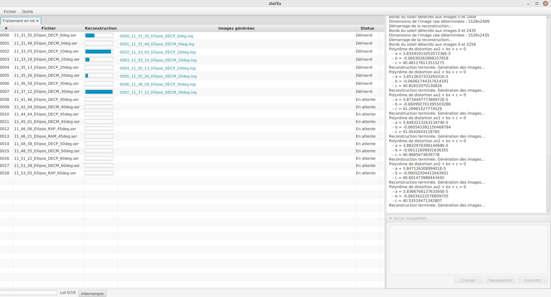
The file list for each SER file will include the log file for each video, as well as all generated images for that SER file.
| In batch mode, we recommend that you pick a custom file name template which will output all images in a single directory: using the sequence number, this will make it easier to import into 3rd party software. |
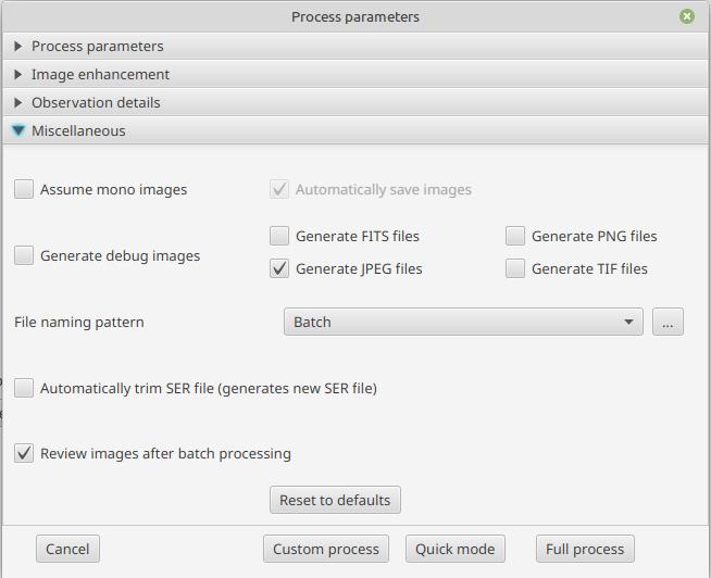
Reviewing batch processed images
Once a batch has been processed, it is possible to review the generated images. This will make it possible, for example, to keep only images with a cloudless disk, or images without distortions.
In order to do so, in the processing options, in the "misc" tab, check the "Review images after batch processing" box:
Once processing is done, a new window will open, allowing you to review the processed images:
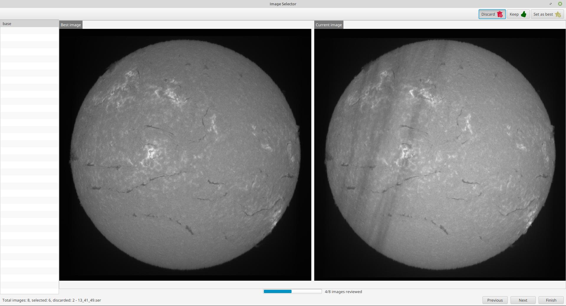
On the top right, you can choose to reject an image, keep it, or set it as the best image. The best image is then displayed on the left, and the current image on the right. You can then compare each image to the best image, and decide whether to keep it or not.
On the left, you have the list of images generated for each SER file. On the bottom right, you can move to the next or previous image, and finish the process.
Once you’re done, the following window will open:
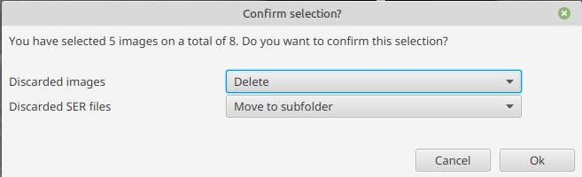
This lets you choose what you want to do with the rejected images: keep them, delete them, or move them to a sub-folder (by default, they will be moved). Similarly, you can choose what you want to do with the SER files which were used to generate these rejected images: keep them, delete them, or move them to a subfolder.
If you use a script in batch mode, the part of the script will only be executed for the images you have kept, which will allow, for example, stacking only the selected images.
Note that in the stack and stack_ref functions, you will then have the possibility to specify the reference selection method manual, which will then choose the best image you have selected.
ImageMath extensions available in batch mode
When you are in batch mode, an additional section is available in ImageMath scripts. This section allows making computations on the results of the processing of each individual image, in order to compose a final image for example (e.g stacking), or to create an animation of several images.
This section must appear at the end of a script and is introduced by the [[batch]] delimiter:
#
# Performs (simple) stacking of images in batch mode
#

[params]
# banding correction width and iterations
bandingWidth=25
bandingIterations=3
# autocrop factor
cropFactor=1.1
# contrast adjustment
gamma=1.2

[tmp]
corrected = fix_banding(img(0);bandingWidth;bandingIterations) (1)
contrast_fixed = auto_contrast(corrected;gamma)                (2)

[outputs]
cropped = autocrop2(contrast_fixed;cropFactor;32)              (3)

# This is where we stack images, simply using a median
# and assuming all images will have the same output size
[[batch]]                                                      (4)
[outputs]
stacked=sharpen(median(cropped)) (5)| 1 | For each SER file, we compute an intermediate corrected image (not stored on disk) |
| 2 | We perform contrast adjustment on the corrected images |
| 3 | Important for stacking: we crop the image to a square centered on the solar disk. The square has a width rounded to the closest multiple of 32 pixels. This is the output of each individual SER file processing. |
| 4 | We declare a [[batch]] section to describe the outputs of the batch itself |
| 5 | An image called stacked will be calculated by using the median value of each individual cropped image |
It is important to understand that only the images which appear in the [outputs] section of the individual file processing are available for use in the [[batch]] section.
Therefore, the cropped image of a single SER file becomes a list of images in the [[batch]] section.
Some functions, like img are not available in the batch mode.
If you need individual images to be available in the batch processing section, then you must assign them to a variable in the [outputs] section:
[outputs]
frame=img(0)       (1)

[[batch]]
[outputs]
video=anim(frame) (2)| 1 | In order to make the img(0) image visible to the batch section, we must assign it to a variable that we call frame |
| 2 | An animation is created using each frame |
Standalone scripts
An additional way to benefit from scripting is to reuse the results of previous sessions (typically, images produced in one or many previous sessions) without having to process a new video.
To do so, you must open the "Tools" menu and select "ImageMath editor".
The interface which pops up is exactly the same as when you are processing a single video, or a batch of files.
The main difference is how images are loaded.
In this mode, you must use either the load or the load_many function to load images, instead of the img function.
| If you use this mode, it is important to load images saved in previous sessions with the FITS format. These files include metadata such as the detected ellipse (solar disk), process parameters, etc. which will permit applying the same functions as you do in a standard processing session. |
Measurements
Redshift Measurements
If you process an H-alpha image, JSol’Ex can automatically search within the image for regions where the redshift (red or blue shift) is particularly strong.
To do this, you must either select the "complete" mode during processing or check the "Redshift Measurements" box in the custom image selection.
The measurements will be valid only if the specified pixel size is correct and you are using a Sol’Ex (other spectroheliographs have different focal lengths).
During processing, an additional image will be generated with the regions outlined in red and the associated speed.
Additionally, if you select the debug images, the parts of the spectrum that allowed finding these regions will be displayed.
Finally, once the detection is complete, you can generate 2 new types of renderings by going to the "Redshift" tab:
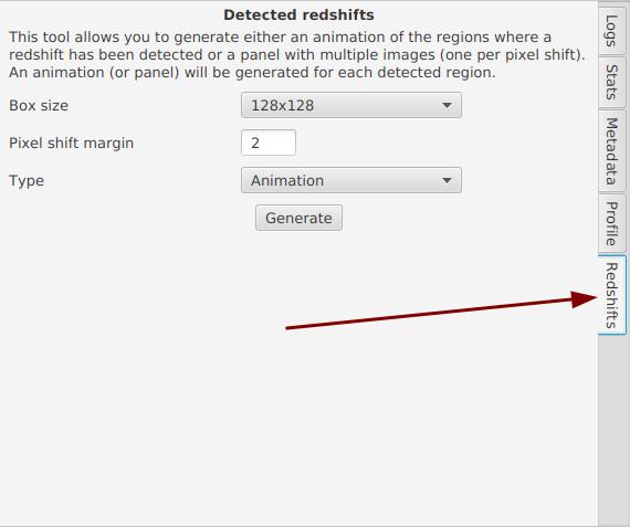
The size corresponds to the minimum size of the region to capture, in pixels. A small region will be centered around the detected filament, but it may be quite pixelated in some cases. The margin allows you to choose how many pixels to offset from what JSol’Ex detected. For example, JSol’Ex might find a maximum shift of 20 pixels, but you may wish to add 2 or 4 pixels of margin for an animation to clearly see the filament appear.
Finally, select the type of rendering:
-
Animation: generates a video where each frame is shifted by 0.25 pixels
-
Panel: generates a single image, a panel where each cell corresponds to a different pixel shift
Measurements thanks to the video analyzer
JSol’Ex provides a tool which will let you see what the detected spectral line is for a particular video. This tool chan be used, for example, to efficiently determine the pixel shift to apply when processing an Helium video.
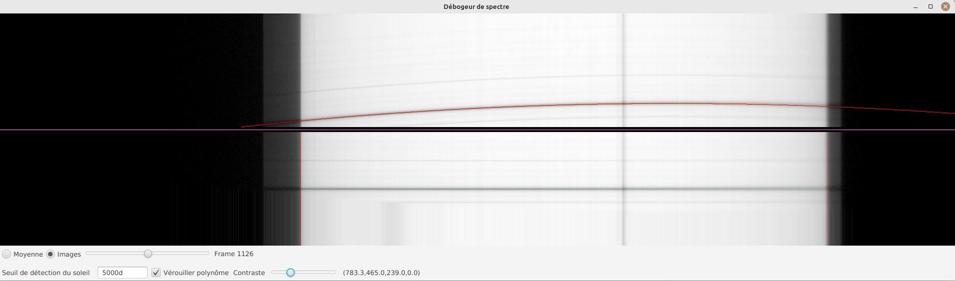
To do this, open the "Video analyzer" in the "Tools" section. Select a video, the tool will compute the average image then show this window:
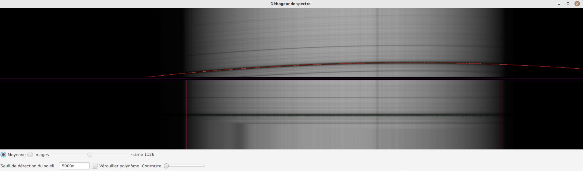
In the upper side you can see the reconstructed average image. The red line is the detected spectral ray, which is built by figuring out the darkest points of the lines. Below the violet line, you can see a geometry corrected version of the average image. If the line was properly detected, then the corrected image should show you perfectly horizontal lines.
In the lower part of the interface, you can adjust several parameters:
-
the "average"/"frames" radio buttons will let you choose between displaying the average image or the individual video frames
-
the sun detection threshold is a parameter you should avoid changing, since the software is not designed to override it in any case. It is provided for advanced debugging in case of bad recognition.
-
the "lock polynomial" checkbox will let us lock the current "red line" (a 2d order polynomial) as the one to use in all frames for display. We will use it in the helium ray spectral search below.
-
the "contrast" slider does what it says
Example of application to determine the helium ray pixel shift
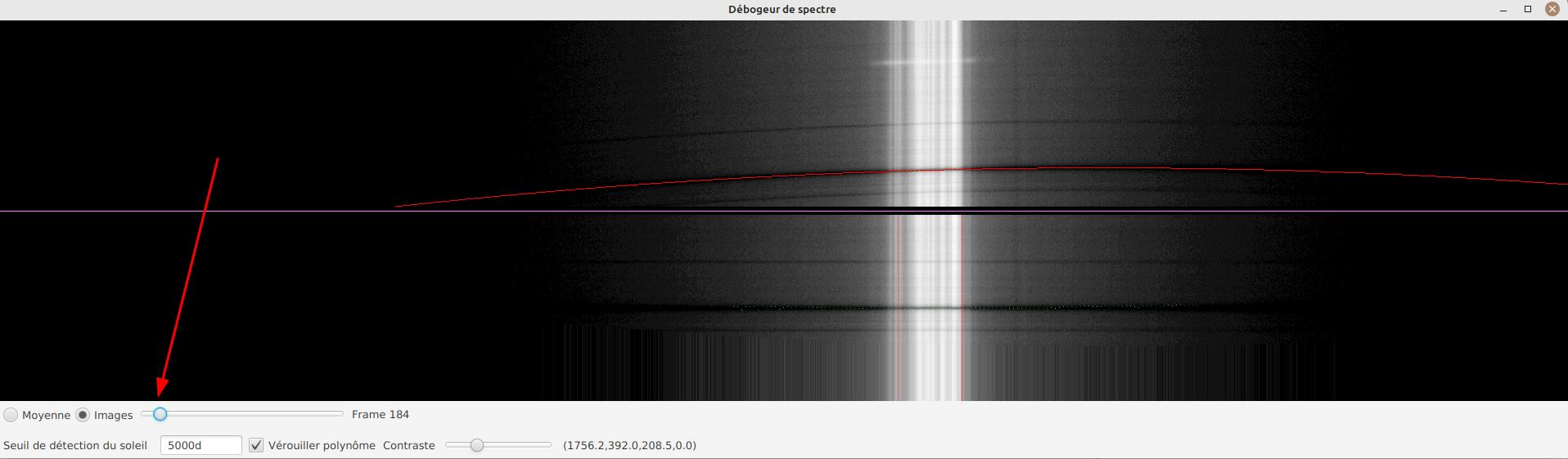
We assume that we have a single SER file which window includes both the helium ray and another ray (e.g sodium) which is dark enough to be detected by JSol’Ex.
We can then proceed by steps:
-
first, lock the polynomial on the average image
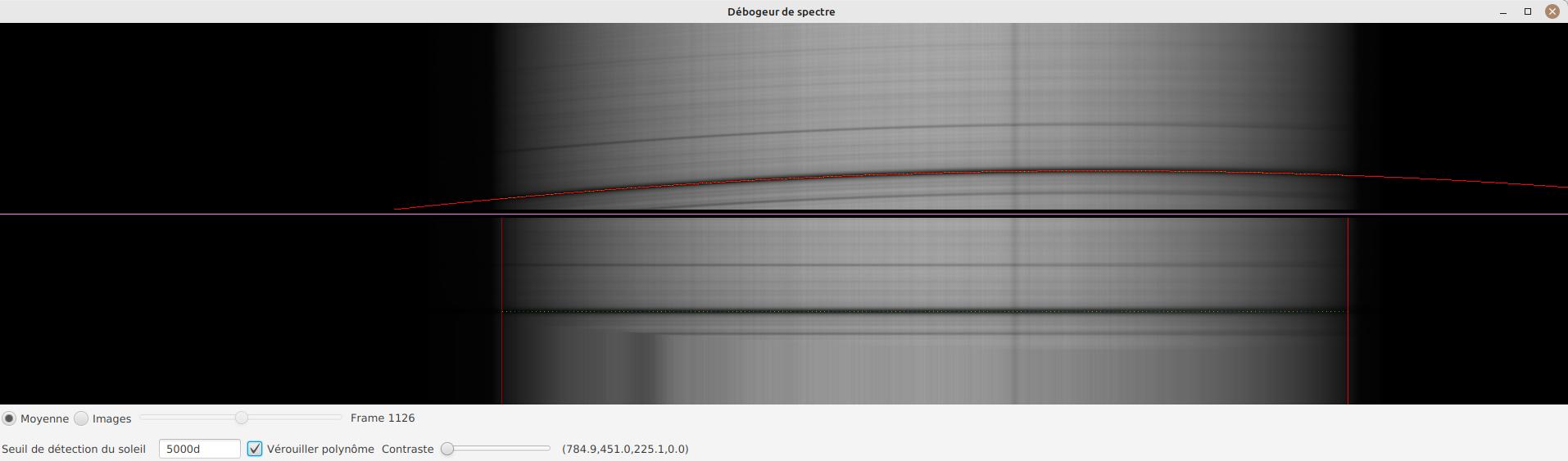
-
select the "Frames" mode
-
Adjust contrast to make the spectrum very bright
-
Select a frame which is close to the sun limb
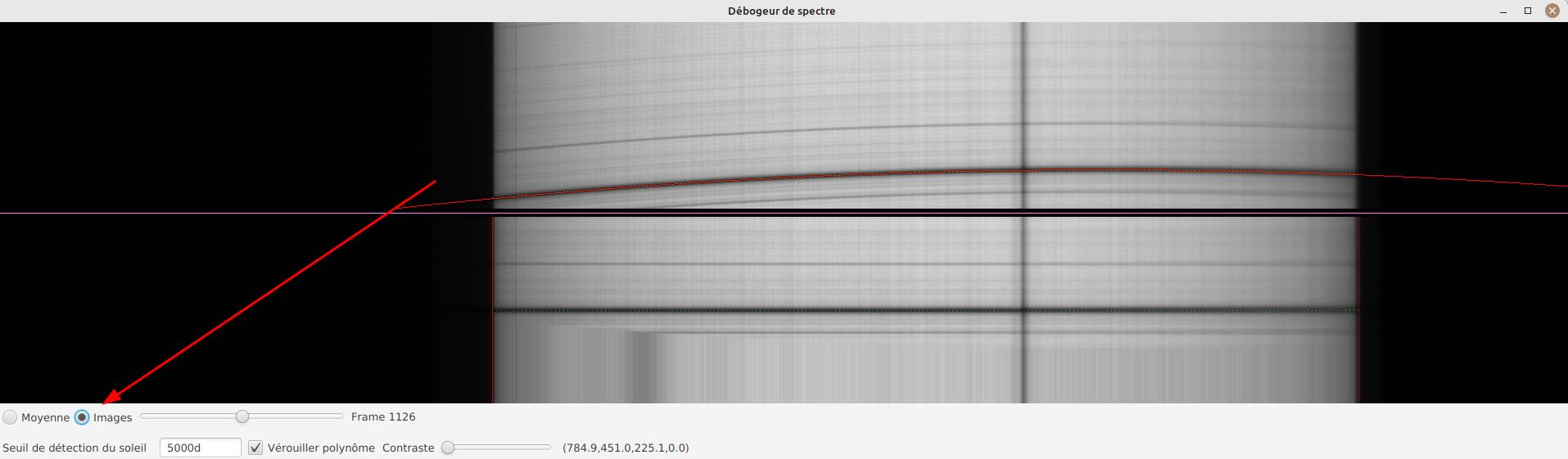
We can now perform measurements: when you are moving the mouse over the image, coordinates are displayed:
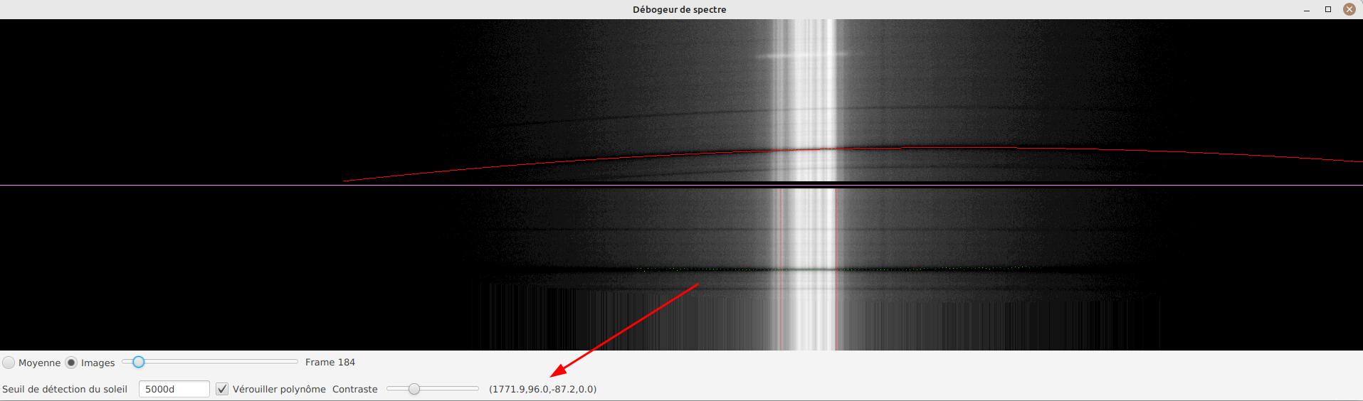
The first 2 numbers are the (x,y) coordinates of the point below the cursor. The 3rd one is the one we’re interested in: it’s the pixel shift between the cursor position and the detected spectral line (in red). The 4th number will let us increase our accuracy by computing an average value from samples.
To add a sample, find a point on the helium line then click on it while holding the CTRL key. You can add as many sample points as you wish.
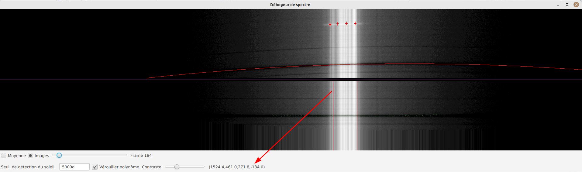
The 4th number is the average of distances and should be a good value to use in your ImageMath scripts. In this example we deduce that the pixel shift is -134.
Stacking and mosaic composition
JSol’Ex provides a tool to stack images and create mosaics. The 2 tools are very similar, but stacking is easier to use. Stacking consists of taking several images of a similar region of the sun and making a single image by aligning the details and averaging the pixels. Mosaics are similar, but they are used to create a single image from several images of different regions of the sun.
The 2 tools are available in the "Tools" menu, then "Stacking and mosaic composition".
The following window will show up:
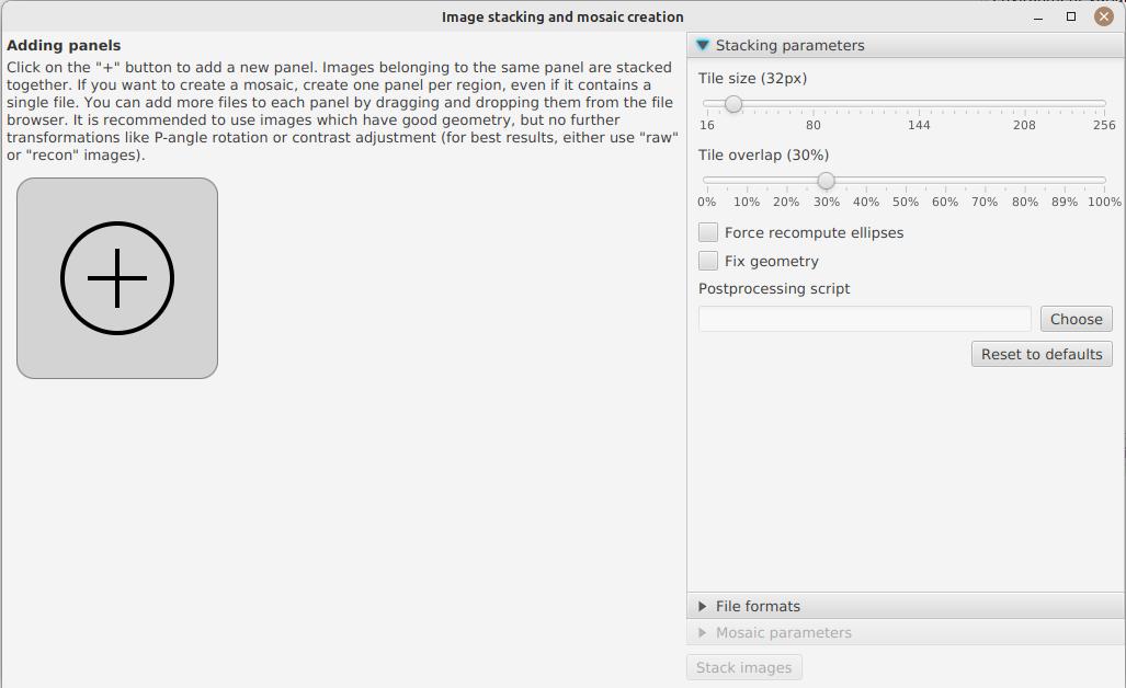
On the left, you can create image panels to stack. If you create a single panel, it will be a simple stacking. If you create several panels, each panel will be stacked, then a mosaic will be composed. A single panel can contain several images, which will be stacked together. To add a panel, click on the "+" button and select the images to stack. Alternatively you can drag and drop one or several images from your file explorer.
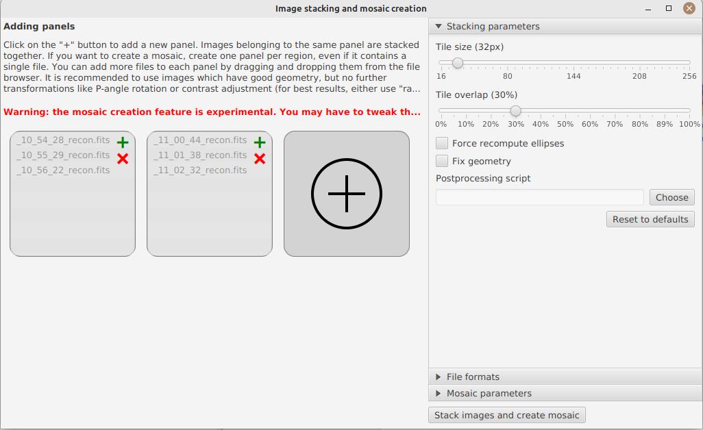
In the image above, we have created 2 panels. The first one contains 3 images which will be stacked to make the north panel, and the second one contains 2 images which will be stacked to make the south panel.
Stacking parameters are visible on the right. It is not recommended to change them, unless you know what you’re doing. The following options are available:
-
the tile size allows to cut the image in tiles for stacking. The smaller the tile size, the more precise the stacking will be, but the longer it will take and the less likely it will be able to compensate for large shifts between images.
-
the sampling factor determines where samples will be picked when computing the distorsion model. A sampling factor of 0.5 combined with a tile size of 32 means that a sample will be picked every 16 pixels.
-
Forcing the computation of ellipses can be useful if the images you import come from another software or if the ellipses were badly detected. In that case, we will recompute them before stacking.
-
Geometry correction should be applied on images which weren’t corrected before (e.g raw images).
The post-processing script is an ImageMath script that you can apply on each of the tiles after stacking.
In a post-processing script, the stacked image is available as image. For example, you can create a script which will apply a deconvolution using the formula rl_decon(image).
|
The other available options let you choose how files are saved. If you have created more than one panel, then the mosaic options become available.
For mosaic composition to work, it is recommended to use raw or recon images, not stretched ones. Indeed, stretched images are more difficult to align.
|
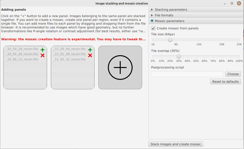
Should you only want to stack images without creating a mosaic, you can disable the "Create mosaic" option. In the other case, you can tweak some parameters, but it is strongly recommended not to change them unless the images you get after sticking are deformed or not reconstructed at all.
Again, you can apply a post-processing script to the mosaic.
Optimal exposure calculator
In the "tools" menu, you will find the optimal exposure calculator. This calculator will determine the optimal exposure time, in order to achieve a perfectly circular sun disk and avoid undersampling.
Enter the following parameters:
-
the camera pixel size (in microns) and the binning
-
the focal length of your instrument
-
the scan speed (a multiple of sideral speed, e.g 2, 4, 8, …)
-
the observation date
The software will then automatically compute the recommended framerate and the optimal exposure time in milliseconds.
Note that you can change the type of spectroheliograph used, which can change the calculation of the optimal exposure.
Spectrum Browser
The Spectrum browser is available in the "Tools" menu. It allows you to visualize the aspect of the spectrum as it would be seen in capture software such as SharpCap or FireCapture.
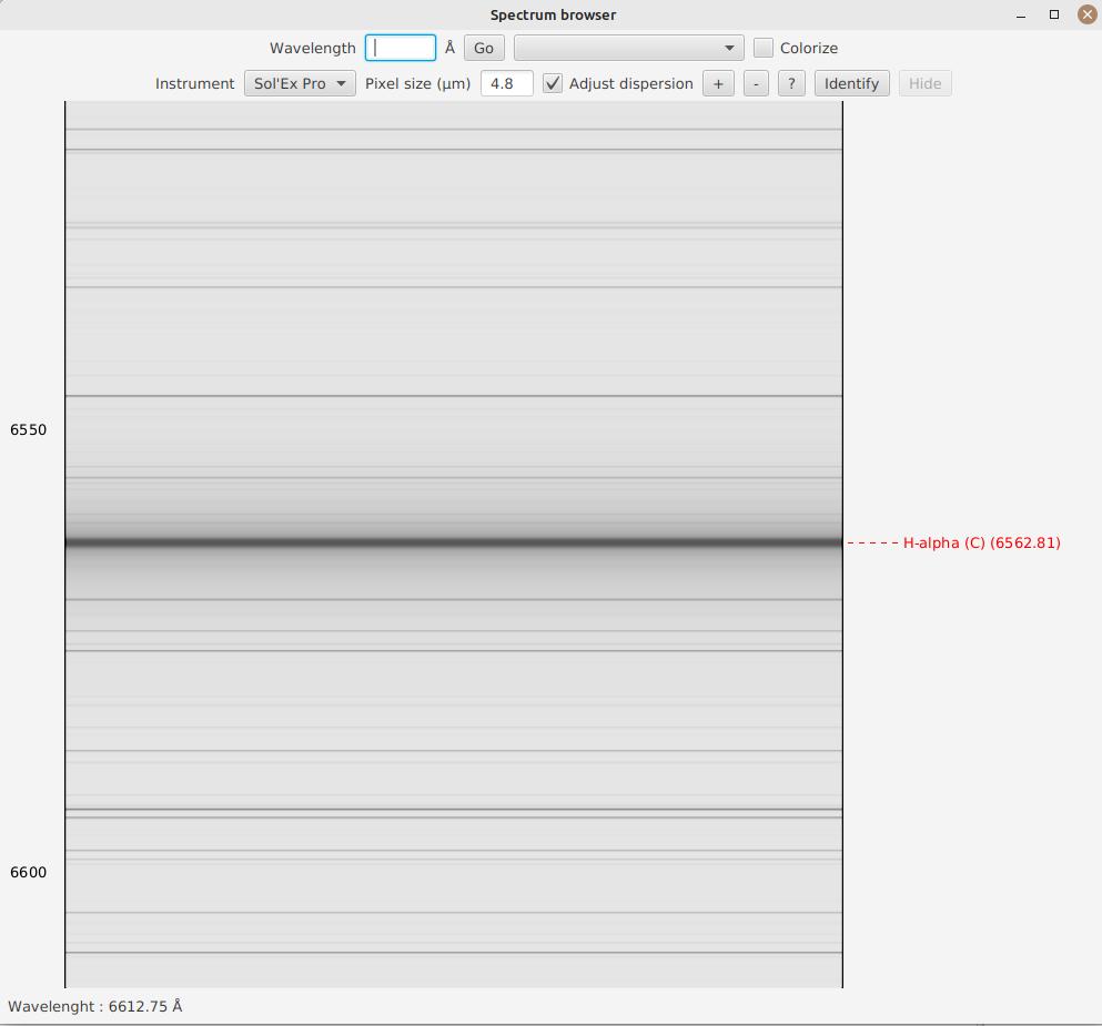
In the "Wavelength" box, you can enter a wavelength in Angstroms. By clicking "Go" or pressing enter, the spectrum will automatically center around this wavelength:
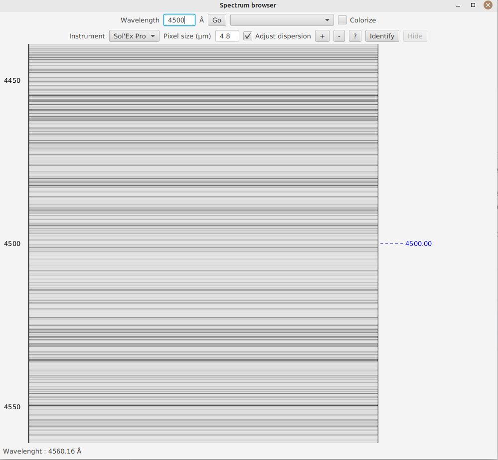
A blue dashed line is added, allowing you to clearly identify the line.
Alternatively, you can directly search for a notable spectral line by selecting it in the box next to the "Go" button.
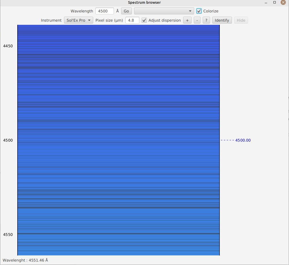
When you click "Colorize", the spectrum is then colorized to give you an idea of where you are in the visible spectrum (however, we recommend staying in grayscale to precisely identify a line):
On the second line, you have the option to choose the spectroheliograph that is used (this will affect the calculated spectral dispersion), as well as to specify the pixel size (remember to multiply by the binning).
If you check the "Adjust Dispersion" box, the spectrum’s dimension is automatically adjusted to precisely match the calculated dispersion per pixel.
You can zoom either by clicking the "+" and "-" buttons, or more simply by pressing "CTRL" and scrolling your mouse wheel. If you zoom, the automatic adjustment is disabled (since it no longer corresponds to the exact dispersion per pixel).
Automatic Identification
Finally, JSol’Ex offers an experimental feature: you can click the "Identify" button to open a file selection window.
Then choose an image of the spectrum, as captured by your software. JSol’Ex will then try to find out which part of the spectrum it is in:
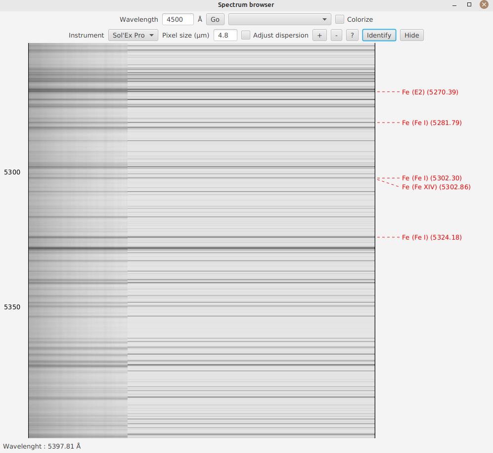
If the identification works, your image will be displayed in transparency, overlaid on the spectrum, on the left side of the image, allowing you to easily verify if the identification was successful.
You can hide the transparent image by clicking the "Hide" button.
Embedded Web Server
In the "Tools" menu, you will find the option to start an embedded web server. This server allows you to view images processed by the software from other computers, by connecting to this server.
This feature can be particularly useful during public presentations, with one computer using JSol’Ex for image acquisition and another computer on the same network for projection on a screen.
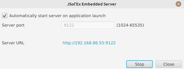
You can configure the port on which the server listens and have the option to start it automatically when the software starts.
The web UI gives access to images being processed as well as their history, in case you process several images successively.
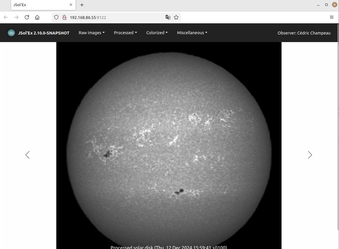
Acknowledgements
-
Christian Buil for designing Sol’Ex and leading the community with great expertise
-
Valérie Desnoux for her remarkable work on INTI
-
Jean-François Pittet for his bug reports, test videos, and geometric correction formulas
-
Sylvain Weiller for his intensive beta-testing, valuable feedback, and processing ideas
-
Ken M. Harrison for improved exposure time calculations
-
Minh Trong Nguyen for his suggestions of improvements and his work on the SHG 700