JSol’Ex

JSol’Ex is a solar images processing software for Christian Buil’s Sol’Ex. It is capable of processing SER files captured with this instrument in order to produce images of the solar disk, in a similar way to what INTI from Valérie Desnoux is doing. It is primarily designed to process images for Sol’Ex, but it might work properly for other kinds of spectroheliographs.

JSol’Ex is free software published under the Apache 2 software license. It is written in en Java and provided for free without any warranty.

Downloads

JSol’Ex can be downloaded from this page. Installaters are available for Linux, Windows and MacOS.

Alternatively, you may run JSol’Ex by checking out the sources and running the following command:

./gradlew jsolex:run

Processing a video file

JSol’Ex only supports SER files, please make sure to configure your capture software to use this format. The main window looks like this:

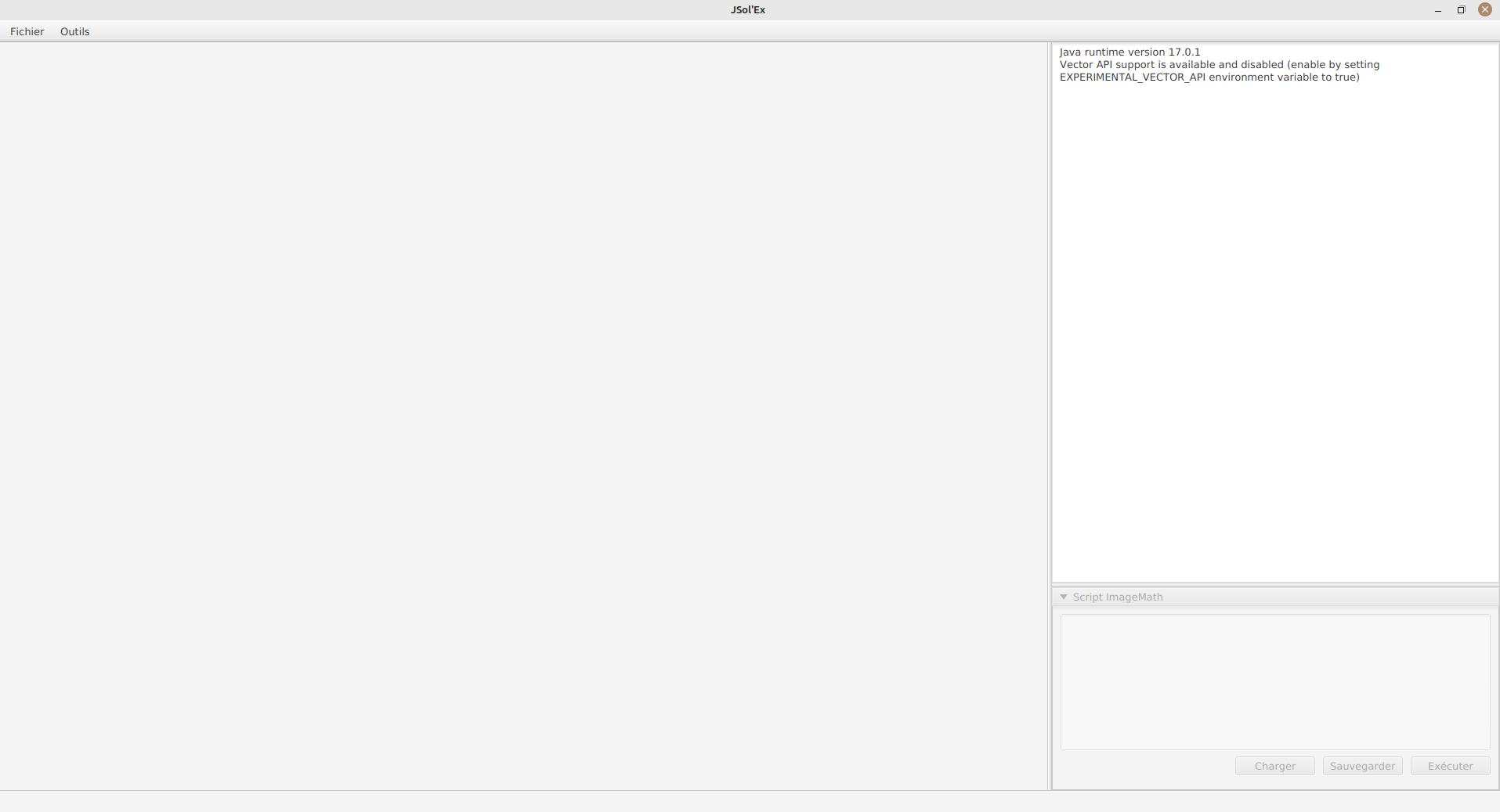
In the "File" menu, choose "Open SER File" and select a file. The following popup should open:

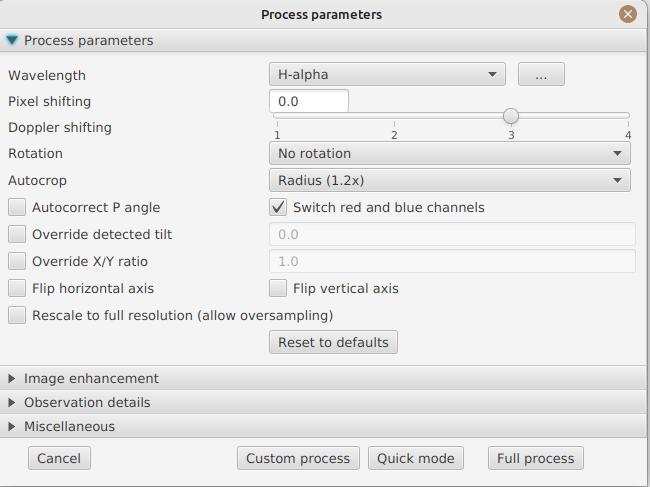
This window is the main entry point for the process parameters. You can specify:

the observation bandwidth: while it’s not mandatory to select that field, doing so will enable automatic colorization of the images. Should your observation bandwidth not be available in the list, you can add more by clicking on the "…" button.
Pixel shift : by default, the software will identify the darkest line in the image and model it as a second order polynomial. Then the image is reconstructed by picking the center of the line, which corresponds to a shift of 0. By using a different shift value, you can produce an image which is "off center", for example to produce images of the solar continuum or to select a different wavelength which isn’t the darkest, such as when observing in helium for example
the Doppler shift is only used when you are observing in h-alpha. JSol’Ex will produce a couple more images shifted in one direction and the other in order to produce a Doppler image. By default, a shift of 3 pixels is used but you can override that parameter.
Rotation : allows performing a left or right rotation (90 degrees) of the images. This can be useful for scans performed in declination, to fix the orientation. This parameter doesn’t affect images produced with ImageMath.
Autocrop : allows automatic cropping of images after geometric transformation. There are multiple modes:
- Off: no autocrop (this is the default)
- Original width: the image will be cropped to a square which width corresponds to the width of the original SER file. Ideal for full solar disks.
- Radius (x…) : the image will be cropped or rescaled to a factor of the determined solar radius. This can be useful for example with truncated disks, if you want to "see" where it would be positioned.
Autocorrect P angle: when checked, the solar angle P will be computed from the observation date (available in the SER file). The generated images will be automatically corrected so that the North is at the top. This parameter will not affect images generated via ImageMath, which need to perform their own correction.
Force tilt: the software is fitting an ellipse around the solar disk which is reconstructed, and uses that information to perform geometric correction. It is possible that the tilt detection is wrong, in which case you can force a value.
Force X/Y ratio: similarly, the X/Y ratio which is detected may be inaccurrate, in which case you can force it to a particular value.
Horizontal and vertical inversion let you mirror the image so that you match the North and East as expected in the output images.
Rescale to full resolution: can be used if your video is oversampled, which typically happens if you are scanning at lower rates (e.g sideral) and that you want to resize the generated image to its full resolution.

Enabling full resolution can lead in significantly larger images and very high memory pressure. It is not recommended to enable this flag.

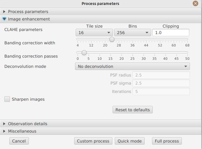
Image enhancement

This section lets you configure the transformations which will be applied to images in order to improve their aesthetic aspect.

CLAHE parameters : allows configuring the CLAHE constrast improvement algorithm. It is possible to configure the size of the tiles used to compute histograms, the histogram resolution and the clipping factor.

Next come the banding correction parameters, which allow to correct transversal bands which can appear on images, for example because of dust on the slit.

Banding correction width: this is the width of the bands which are used in the transversallium correction algorithm. Bands are used to compute the average brightness of pixels in the band, then lines are corrected according the band they belong to.
Banding correction passes: the more passes you’ll apply, the more lines should be corrected, at the cost of lower constrast images

Another section lets you configure image deconvolution. By default, no deconvolution is applied, but you can choose the deconvolution algorithm and its parameters.

For the Richardson-Lucy deconvolution, you can choose the size of the synthetic PSF, the sigma factor and the number of iterations.

Finally, you can choose to apply a detail enhancement filter at the end of the processing by checking the "sharpen images" box.

Observation parameters

Observation parameters are used to insert metadata into FITS files. As of now, we do not recommend to publish images produced using JSol’Ex to the BASS2000 database because the FITS header that this software uses are not validated against what the database expects.

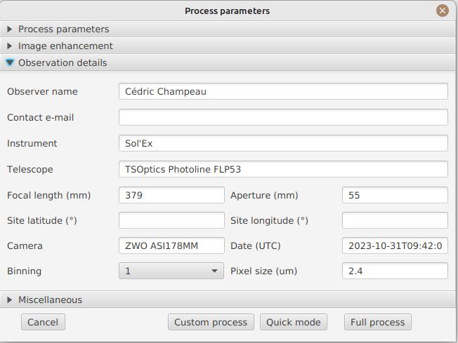
Here are the fields available in JSol’Ex:

Observer : the person who made the observation
Email : the email address of the person who made the observation
Instrument : pre-filled to "Sol’Ex"
Telescope : your telescope or refractor used with the Sol’Ex instrument
Focal length and aperture of the telescope
Latitude and longitude of the observation site
Camera
Date : pre-filled with information from the SER file, expressed in the UTC timezone
Binning : the binning of pixels when the video was recorded
Pixel size : the size of the camera pixels in microns

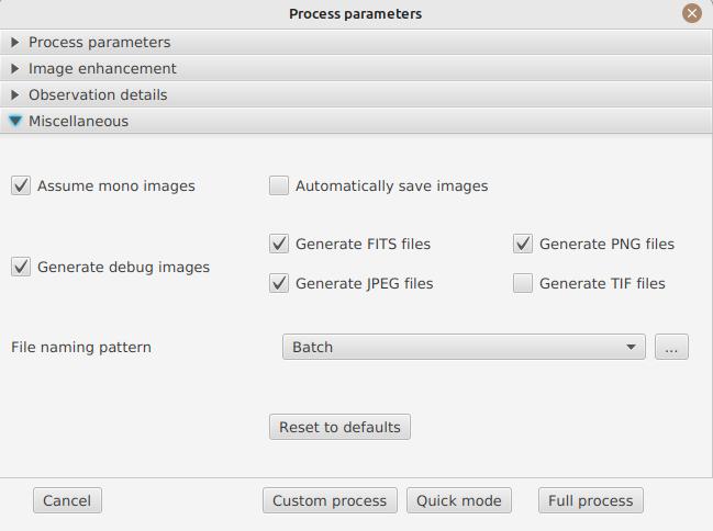
Other parameters

Assume mono video : when checked, JSol’Ex will not try to perform demosaicing of the video, by assuming it’s a mono one. This can considerably speedup processing, and because most videos for Sol’Ex will be mono, it is better to leave this checked.
Automatically save images : if checked, all images which are generated by the software will be saved to disk immediately. If unchecked, then it’s your responsibility to save them by clicking on the "save" button of each image tab.
Generate debug images: when checked, additional images will be generated to highlight edge detection, tilt detection and average image. These can be useful to figure out what when wrong when the software doesn’t produce the expected results.
Generate FITS files : in addition to PNG files, will also generate FITS files.

File naming patterns

By default, JSol’Ex will output the generated images in a subfolder which name matches the name of the SER file (without extension). Then each kind of images is stored in a subdirectory of that folder (e.g raw, debug, processed, …). If that naming convention doesn’t suit you, you can create your own naming patterns, by clicking the "…" dots:

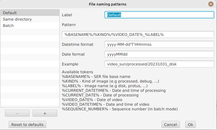
A naming pattern consists of a label, but more importantly a pattern consisting of tokens delimited by the % character.

Please find below the list of available tokens:

%BASENAME% is the SER file base name, that is to say the name without extension
%KIND% is the kind of images (raw, debug, processed, …)
%LABEL% is the label of the produced images, e.g recon, protus
%CURRENT_DATETIME% is the date and time of processing
%CURRENT_DATE% is the date of processing
%VIDEO_DATETIME% is the date and time of the video
%VIDEO_DATE% is the date of the video
%SEQUENCE_NUMBER% is the sequence number in case of batch processing (4 digits, eg. 0012)

This for example would be a pattern which puts all generated files in a single folder:

%BASENAME%/%SEQUENCE_NUMBER%_%LABEL%

The "example" field shows you what the generated file names would look like.

Process start

JSol’Ex provides 3 processing modes: quick, full and custom.

The "quick" mode will only produce a couple images: the raw reconstructed one, and a geometry corrected version. It is useful in your initial setup, when you’re still trying to figure out the tilt or exposure, for example. It is recommended to combine this mode with not saving images automatically, so that you don’t fill your disk with images that you will never use.
The "full" mode will generate all images that JSol’Ex can automatically produce:
the raw, reconstructed image
a geometry corrected and color-stretched version
a colorized image, if the bandwidth you have selected provides the required parameters
a negative image version
a virtual eclipse, to simulate a coronagraph
a mixed image combining the colorized version with the virtual eclipse
a Doppler image
the "custom" mode will let you precisely pick which images you want to generate. It even provides a more advanced mode letting you script generated images, allowing the generation of images which weren’t designed initially (see the section about custom images).

Image display

Once images are generated, they appear one after each other in tabs. These tabs provide you with the ability to tweak the contrast of images and save them, typically when you unchecked the automatic save option.

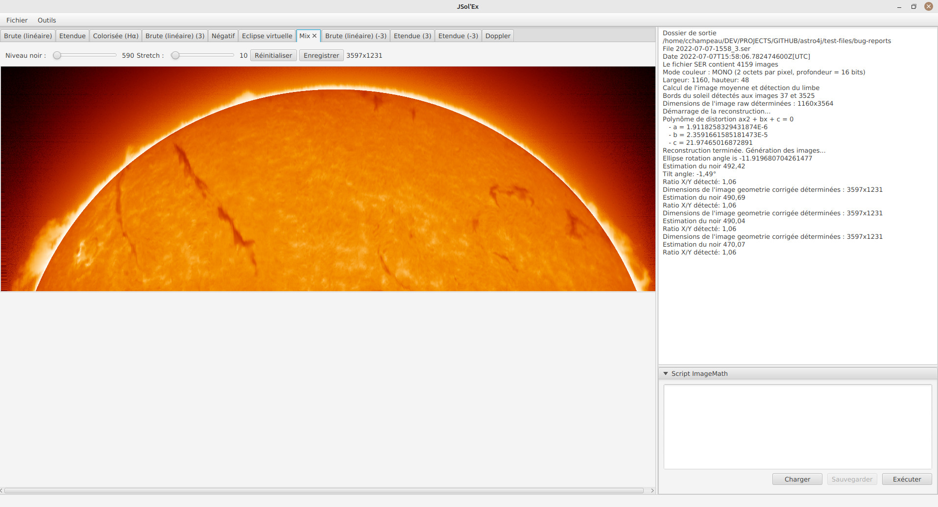
It is possible to zoom into the images by using the mouse wheel. In addition, right-clicking the image will let you open it into your file explorer or in a separate window.

Watching a directory for changes

When trying to find the ideal focus, it can be useful to process video files quickly until we obtain a satisfying result. JSol’Ex offers an easy way to do this, by watching the changes in a directory : new videos which are saved in that directory will immediately be processed.

To do this, in the file menu, choose "Watch directory" then select the directory where your SER files will be recorded (e.g the output directory of SharpCap).

JSol’Ex will switch to watch mode, which you can interrupt by clicking the button which appeared in the bottom left of the interface.

Now, open your capture software and record a new video. Once it’s done, switch to JSol’Ex : it will open the process parameters configuration window. Select your processing parameters then start the processing.

Once you have the result, switch back to your capture software and acquire a new video. Once its done, switch back to JSol’Ex: this time, the process parameters window won’t open, because it’s going to reuse the parameters from the first video, allowing to process new videos very quickly!

Make sure that when you switch from your capture software to JSol’Ex that the recording is finished. If not, processing can start on an incomplete file and fail.

Once you’re happy with the result, click on the "Stop watching" button on the bottom left.

You can combine the watch mode with opening an image in a new window (by right-clicking on an image, you can open it in a new window). When a new SER file will be processed, the corresponding image will automatically replace the one in the external window. This can be useful in demonstrations, if you have for example a separate monitor where you would only show the result of processing.

Customization of generated images

When you click the "custom" mode instead of the quick or full ones, JSol’Ex provides you with an interface which will let you declare exactly what should be output.

There are 2 modes available: the simple one and the ImageMath one.

In the simple one, you can pick which images to generate by clicking the right boxes. It is also possible to ask for the creation, in parallel, of images at different pixel shifts.

For example, should you want to generate images from the continuum to the observed ray, you can enter -10;-9;-8;-7;-6;-5;-4;-3;-2;-1;0;1;2;3;4;5;6;7;8;9;10 which will have the consequence of generating 21 distinct images ranging from shift -10 to +10. This can be particularly useful if you want, for example, to generate an animation.

It’s worth noting that if you check some images like "Doppler", some pixel shifts will be automatically added to the list (e.g -3 and +3).

If this isn’t good enough for you, you can go even more advanced by enabling the "ImageMath" mode which is extremely powerful while relatively simple to grasp.

ImageMath : images generation scripts

Introduction to ImageMath

The "ImageMath" mode is a mode which will let you declare which images to generate by writing small scripts. It relies on a simple script language designed specifically for generating Sol’Ex images.

Let’s illustrate this by going back to our previous example, where you wanted to generate images in the [-10;10] pixel shift range. In the "simple" mode, you had to manually enter all pixel shifts, which can be a little cumbersome. In the "ImageMath" mode, we have a language which will let us to this with a single instruction.

First, select the ImageMath mode in the select box and click on "Open ImageMath". The following interface show up:

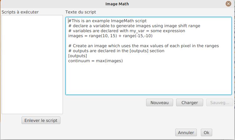
On the left side, "Scripts to execute", you will find the list of all scripts which will be applied in your session.

This is really the list of scripts which are applied in that session, not the list of available scripts! Click on the "remove" button to remove scripts from execution in the session.

Scripts must be saved on your local disk and can be shared with other users. Their contents is editable in the rightmost part of the interface.

Start with removing the contents of the sample script and replace it with:

range(-10;10)

Then click on "Save". Select a destination file and proceed: the script is now added to the list on the left, as being executed in this session.

Click on "Ok" to close ImageMath and only keep the "geometry corrected (stretched)" images. Click on "Ok" to start processing, you will now have the 21 required images generated:

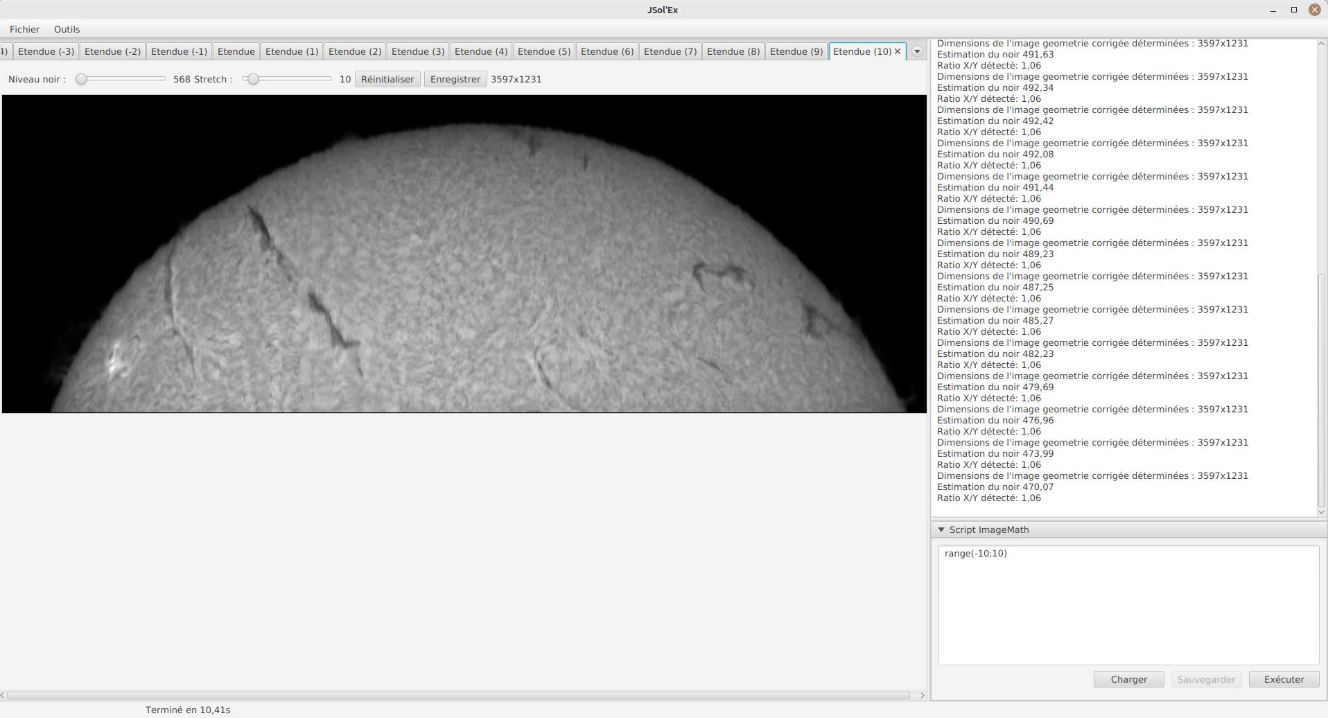
Functions available in ImageMath

For now we’ve only used one function called range, which let us generate about 20 images, but there are many others available.

Base functions:

img requests an image at a particular pixel shift. For example, img(0) is the image centered on the detected spectral ray, while img(-10) is a continuum image, shifted 10 pixels up.
list builds a list from its arguments. e.g list(img(-3), img(3))
avg computes the average of different images. For example: avg(img(-1), img(0), img(1)) computes the average of images at pixel shifts -1, 0 and +1. It is also possible to use the simpler avg(range(-1,1)) expression
max computes the maximum of multiple images, for example max(img(-3), img(3)). Maximum is per pixel.
min computes the minimum of multiple images, for example min(img(-3), img(3)). Minimum is per pixel.
range generates images in a certain range of pixel shifts. It accepts either 2 or 3 arguments. The first 2 are the lower and higher pixel shifts (included). The 3rd, optional one is a step value. For example, using range(-5;5;5) will only generate 3 images at pixel shifts -5, 0 and 5.

You can also perform calculus with images, for example:

(img(5)+img(-5))/2 which is equivalent to avg(img(5),img(-5)).

Another example: 0.8*img(5) + 0.2*avg(range(0;10))

Other functions are available:

invert, generates a color inverted image
clahe performs Contrast Limited Adaptative Histogram Equalization on your image. It supports either 2 or 4 parameters. In the first form, it takes the image to equalize and clip factor, for example: clahe(img(0); 1.5). In the long form, it takes 2 additional parameters which are the tile size (used to compute histograms) and the number of bins (the lower, the smaller the dynamic range). e.g clahe(img(0); 128; 256; 1.2)
adjust_contrast applies simple contrast adujstment by clipping values under the minimal value or above the maximal value. e.g adjust_contrast(img(0), 10, 210). The range is must be between 0 and 255.
asinh_stretch applies the inverse arcsin hypobolic transformation to increase constrast. It accepts 3 arguments: the image, the black point value and a stretch value.
linear_stretch expands the image dynamic range. It takes either one or 3 arguments: the image and optionally the minimal and maximal value. The min/max values are used to determine to what range to expand. It’s a 16-bit value between 0 and 65535. For example: linear_stretch(img(0))
fix_banding applies the banding correction algorithm. It accepts 3 arguments: the image, the banding width, the number of passes. For example, fix_banding(img(0), 10, 5).

If you don’t want to provide a custom black point value, you can use a predefined one, which is estimated from the image. It is available as the blackPoint variable, e.g asinh_stretch(img(0), blackPoint, 100)

crop will perform arbitrary cropping of an image. This function takes 5 parameters: the coordinates of the top left point, then the width and height of the desired image. For example: crop(img(0), 100, 100, 300, 300).
crop_rect crops the image do the specified dimensions, with the guarantee that the center of the sun disk will be in the center of the new image. For example: crop-rect(img(0), 1024, 1024). This doesn’t perform any scale change: if the target image cannot fit the solar disk, it will be truncated.
autocrop will perform a square cropping of the image. It makes use of the detected ellipse to center the image on the sun center. e.g autocrop(img(0)).
autocrop2 will perform a square cropping of the image, centered on the solar disk, similarly to autocrop, but the dimensions of the cropped image are calculated with a factor of the disk diameter. By default, dimensions of the cropped image are a multiplier of 16. e.g autocrop2(img(0);1.1) will crop around 1.1 times the diameter. autocrop2(img(0);1.1;32) will do the same, but the resulting image will have width and height as multipliers of 32.
colorize triggers colorization of the image. It either takes 2 parameters, the image and a profile name, or 7 parameters. The profile name is the name of the color profile as found in the process parameters. For example: colorize(img(0), "h-alpha"). The long version takes the image and for each RGB color channel, the "in" and "out" values determining the color curves, in the 0..255 range. e.g `colorize(img(0), 84, 139, 95, 20, 218, 65) is strictly equivalent to the h-alpha version. It’s worth noting that colorizing is highly sensitive to the source pixel values. It may be required to run an asin_stretch function before colorizing.
remove_bg performs background removal on an image. This can be used when the contrast is very low (e.g in helium processing) and that stretching the image also stretches the background. This process computes the average value of pixels outside the disk, then uses that to perform an adaptative suppression depending on the distance from the limb, in order to preserve light structures around the limb. For example: remove_bg(stretched). Another variant lets you specify a tolerance value: remove_bg(stretched, 0.2). The lower the tolerance, the weaker the correction will be.
rgb creates an RGB image by associating mono images on the respective R, G and B channels. As a consequence it accepts 3 parameters, for exemple: rgb(img(3), avg(img(3), img(-3)), img(-3)).
saturate (de)saturates an RGB image. It takes 2 arguments : an RGB image and a saturation factor (relative to the current image saturation). e.g: saturate(doppler, 2).
anim allows the creation of MP4 files from your individual frames. It takes a list of images as the first parameter, and an optional delay (default 250ms) between frames as 2d parameter. e.g anim(range(-5;5)). Warning: animation creation is a resource intensive operation.
load loads an image from the file system. It takes the path to the file as an argument. For example: load("/path/to/some/image.png"). Instead of using an absolute path, it is possible to use workdir in combination.
load_many allows loading several images at once from a directory. For example: load_many("/path/to/folder"). An optional parameter lets you specify a regular expression to filter images: load_many("/chemin/vers/dossier", ".*cropped.*").
workdir sets the default working directory, which is used whenever the load operation is done with relative paths. e.g workdir("/path/to/session")
rl_decon applies theRichardson-Lucy deconvolution algorithm to the image. This function makes use of a synthetic PSF. It requires a single mandatory parameter which is the image to process. For example: rl_decon(img(0)). 3 optional parameters are available: the PSF radius in pixels, the sigma factor and the number of iterations. For example: rl_decon(img(0), 2.5, 2.5, 10).
sharpen will apply sharpening the target image. For example, sharpen(img(0)).
blur will apply Gaussian blur the target image. For example, blur(img(0)).
disk_fill will fill the detected sun disk with a fill color (by default, the detected black point). e.g disk_fill(img(0)) or disk_fill(img(0), 0).
rescale_rel rescales an image. It accepts 3 arguments: the image, then the scaling factors for X and Y. For example, rescale_rel(img(0);2;2) will double the size of an image.
rescale_abs rescales an image to the specified dimensions. It takes 3 arguments: the image then the desired width and height. For example, rescale_abs(img(0);2048;2048).
radius_rescale is a relative scaling method which can facilitate mosaic composition. It will therefore most likely be used in batch mode. It allows rescaling a set of images so that they all have the same solar disk radius (in pixels). In order to do so, it will perform an ellipse regression against each image to compute their solar disk, then will rescale all images to match the radius of the largest one. For example: radius_rescale(cropped).

Rotation functions:

A special variable named angleP contains the computed solar P angle, from the observation details. It is expressed in radians and can typically be used with the rotate_rad function to perform correction.

rotate_left performs a rotation of the image to the left. For example, rotate_left(img(0)).
rotate_right performs a rotation of the image to the right. For example rotate_right(img(0)).
rotate_deg performs an arbitrary rotation, in degrees. It accepts between 2 and 4 parameters: the image and the rotation angle are mandatory. For example: rotate_deg(img(0), 45). You can then specify the fill value for the pixels which didn’t belong to the original image: rotate_deg(img(0), 45, 800) and last, if you add 1 as the last argument, the image will be rescaled so that all pixels from the original image are found in the rotated version.
rotate_rad performs an arbitrary rotation, in degrees. It accepts between 2 and 4 parameters: the image and the rotation angle are mandatory. For example: rotate_rad(img(0), 0.25). You can then specify the fill value for the pixels which didn’t belong to the original image: rotate_rad(img(0), 0.25, 800) and last, if you add 1 as the last argument, the image will be rescaled so that all pixels from the original image are found in the rotated version.

Decorative functions

draw_globe draws a globe which orientation and diameter matches the detected solar parameters. It takes between 1 and 4 arguments. The 1st one is the image on which to draw the globe. e.g: draw_globe(img(0)). The next, optional parameters are the P angle (in radians), the B0 angle (in radians) and the ellipse. e.g: draw_globe(img(0), p, b0, ellipse).
draw_obs_details prints on the image the observation details. For example: draw_obs_details(img(0)). By default, placed in the top left corner. It’s possible to set the (x,y) position explicitly: draw_obs_details(img(0), 100, 100).
draw_solar_params prints on the image the detected solar parameters. For example: draw_solar_params(img(0)). By default, placed in the top right corner. It’s possible to set the (x,y) position explicitly, for example: draw_solar_params(img(0), 500, 100).

ImageMath scripts

In the previous section, we have seen the building blocks of ImageMath, which permit computation of new images. Scripts go beyond this by combining these into a powerful tool to generate images. As an illustration, let’s look at this script which will let us generate an Helium image. Helium image processing is complicated, because the Helium ray is very dim and the software cannot find it in the image. Therefore, we can use a technique which consists of taking a larger capture window which includes a dark ray, then by determining by how many pixels the helium ray is shifted from that line, we can reconstruct an image. Even so, the work is not finished, since it’s an extremely low constrast ray, so we have to substract the continuum value. Producing such images is quite cumbersome but can be simplified to the extreme with ImageMath:

[params]
# Pixel shift of the helium ray
HeliumShift = -85
# Hi and lo values of the continuum (pixel shifts)
ContinuumLo=-80
ContinuumHi=-70
# Continuum substration coefficient
ContinuumCoef=0.95
# Arcsinh image strech
Stretch=10
# Banding width
BandWidth=25
# Banding correction iterations
BandIterations=10

## Tmp variables
[tmp]
continuum = max(range(ContinuumLo,ContinuumHi))
helium_raw = autocrop(img(HeliumShift) - ContinuumCoef*continuum)

## Now the output images!
[outputs]
helium = asinh_stretch(helium_raw, blackPoint, Stretch)
helium_fixed = asinh_stretch(fix_banding(helium_raw;BandWidth;BandIterations),blackPoint, Stretch)
helium_color = colorize(helium_fixed, "Helium (D3)")

Our script consists of 3 different sections: [params], [tmp] and [outputs]. The only mandatory section is the [outputs] one: it defines which images we want to have in the end. The name of all other sections is arbitrary, you can create as many sections as you want.

Here, we defined a [params] section which highlights which parameters we want users to be able to tweak for their needs. This is where we find the value of our helium ray pixel shift (-85).

A variable can only contain ASCII characters, digits (except for the 1st character) or the _ character. For example, myVariable, MyVariable or MyVariable0 all all valid identifiers. hélium is invalid (because of the accent).

Variables can be used in other variables or function calls.

Variables are case sensitive. myVariable et MyVariable are 2 distinct variables!

Our 2d section, [tmp], defines intermediate images we want to work with, but for which we don’t care about seeing the result. Here we have 2 intermediate images: one of the continuum, which uses a max of the continuum range, and a "raw" helium image which is the reconstructed image, substracted with the continuum one.

Last but not least, the [outputs] section declares the images we want to generate:

helium = asinh_stretch(helium_raw, blackPoint, Stretch) will create an image with the helium label, which is simply a stretched version of our raw helium image.

The expression helium_fixed = asinh_stretch(fix_banding(helium_raw;BandWidth;BandIterations),blackPoint, Stretch) does something similar, but actually performs a banding correction in addition.

Last, helium_color = colorize(fix_banding(helium_raw;BandWidth;BandIterations), "Helium (D3)") generates a colorized version of the image.

Comments can be added either with the # or // prefix.

Batch processing

In addition to single SER file processing, JSol’Ex provides a batch mode. In this mode, several videos are processed in parallel, which can be extremely useful if you want to generate many images to be used in external software like AutoStakkert!.

To start a batch, in the file menu, choose "batch mode". Select all the files you want to process (they need to be in the same directory), then the same parameters window as in the single mode will pop up. This window will let you configure the batch processing, but there are subtle differences:

you can only select a single ray for all videos, they must all be the same
the "automatically save images" parameter is always set to true
images will not show up in the interface, but will be shown in a table instead

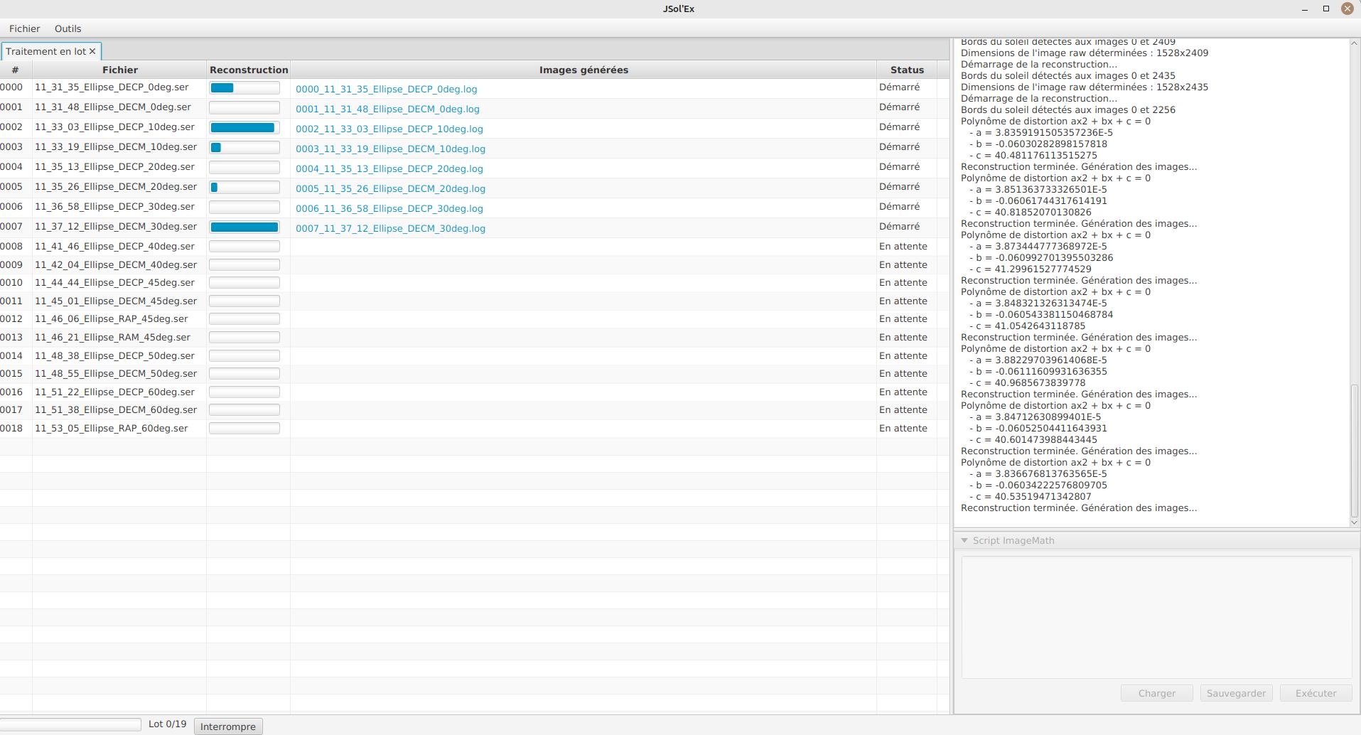
The file list for each SER file will include the log file for each video, as well as all generated images for that SER file.

In batch mode, we recommend that you pick a custom file name template which will output all images in a single directory: using the sequence number, this will make it easier to import into 3rd party software.

ImageMath extensions available in batch mode

When you are in batch mode, an additional section is available in ImageMath scripts. This section allows making computations on the results of the processing of each individual image, in order to compose a final image for example (e.g stacking), or to create an animation of several images.

This section must appear at the end of a script and is introduced by the [[batch]] delimiter:

#
# Performs (simple) stacking of images in batch mode
#

[params]
# banding correction width and iterations
bandingWidth=25
bandingIterations=3
# autocrop factor
cropFactor=1.1
# contrast adjustment
clip=.8

[tmp]
corrected = fix_banding(img(0);bandingWidth;bandingIterations) (1)
contrast_fixed = clahe(corrected;clip)                         (2)

[outputs]
cropped = autocrop2(contrast_fixed;cropFactor;32)              (3)

# This is where we stack images, simply using a median
# and assuming all images will have the same output size
[[batch]]                                                      (4)
[outputs]
stacked=sharpen(median(cropped))                               (5)

1	For each SER file, we compute an intermediate corrected image (not stored on disk)
2	We perform contrast adjustment on the corrected images
3	Important for stacking: we crop the image to a square centered on the solar disk. The square has a width rounded to the closest multiple of 32 pixels. This is the output of each individual SER file processing.
4	We declare a `[[batch]]` section to describe the outputs of the batch itself
5	An image called `stacked` will be calculated by using the median value of each individual `cropped` image

It is important to understand that only the images which appear in the [outputs] section of the individual file processing are available for use in the [[batch]] section. Therefore, the cropped image of a single SER file becomes a list of images in the [[batch]] section. Some functions, like img are not available in the batch mode. If you need individual images to be available in the batch processing section, then you must assign them to a variable in the [outputs] section:

[outputs]
frame=img(0)       (1)

[[batch]]
[outputs]
video=anim(frame)  (2)

1	In order to make the `img(0)` image visible to the batch section, we must assign it to a variable that we call `frame`
2	An animation is created using each `frame`

Standalone scripts

An additional way to benefit from scripting is to reuse the results of previous sessions (typically, images produced in one or many previous sessions) without having to process a new video.

To do so, you must open the "Tools" menu and select "ImageMath editor". The interface which pops up is exactly the same as when you are processing a single video, or a batch of files. The main difference is how images are loaded. In this mode, you must use either the load or the load_many function to load images, instead of the img function.

If you use this mode, it is important to load images saved in previous sessions with the FITS format. These files include metadata such as the detected ellipse (solar disk), process parameters, etc. which will permit applying the same functions as you do in a standard processing session.

Measurements thanks to the spectrum debugger

JSol’Ex provides a tool which will let you see what the detected spectral line is for a particular video. This tool chan be used, for example, to efficiently determine the pixel shift to apply when processing an Helium video.

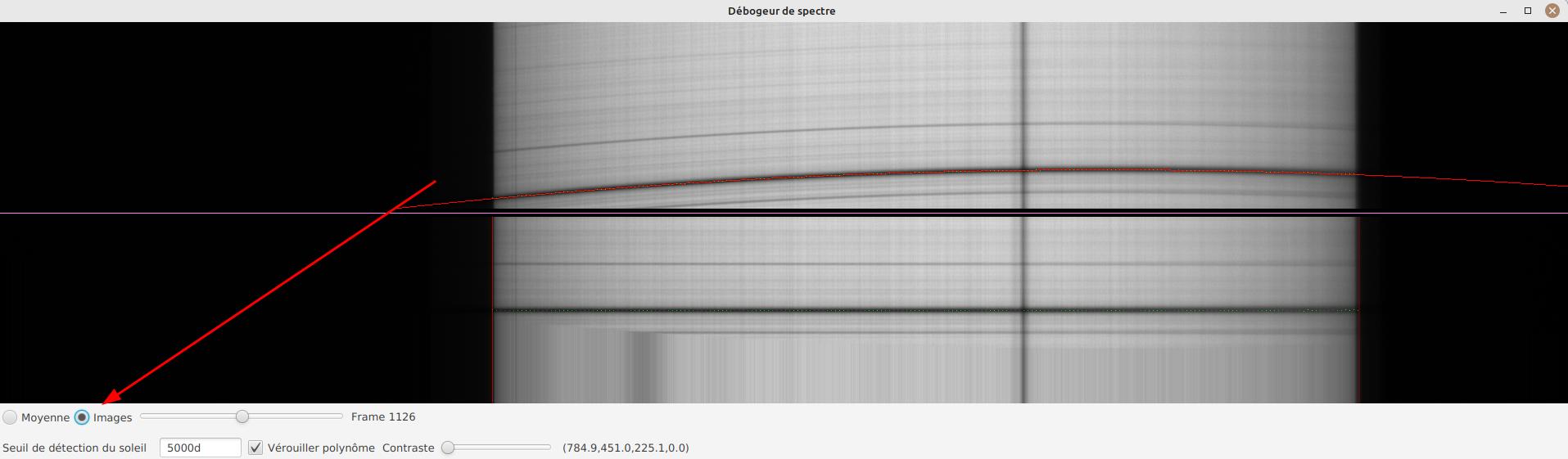
To do this, open the "Spectrum debugger" in the "Tools" section. Select a video, the tool will compute the average image then show this window:

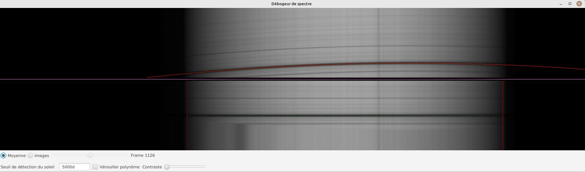
In the upper side you can see the reconstructed average image. The red line is the detected spectral ray, which is built by figuring out the darkest points of the lines. Below the violet line, you can see a geometry corrected version of the average image. If the line was properly detected, then the corrected image should show you perfectly horizontal lines.

In the lower part of the interface, you can adjust several parameters:

the "average"/"frames" radio buttons will let you choose between displaying the average image or the individual video frames
the sun detection threshold is a parameter you should avoid changing, since the software is not designed to override it in any case. It is provided for advanced debugging in case of bad recognition.
the "lock polynomial" checkbox will let us lock the current "red line" (a 2d order polynomial) as the one to use in all frames for display. We will use it in the helium ray spectral search below.
the "contrast" slider does what it says

Example of application to determine the helium ray pixel shift

We assume that we have a single SER file which window includes both the helium ray and another ray (e.g sodium) which is dark enough to be detected by JSol’Ex.

We can then proceed by steps:

first, lock the polynomial on the average image

select the "Frames" mode

Adjust contrast to make the spectrum very bright

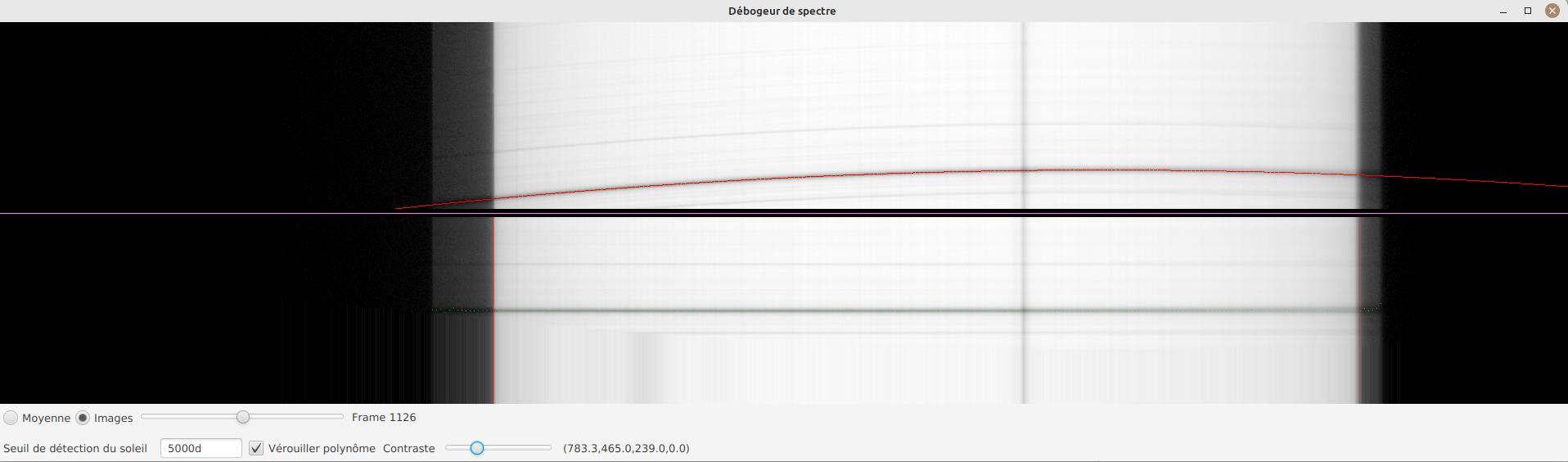
Select a frame which is close to the sun limb

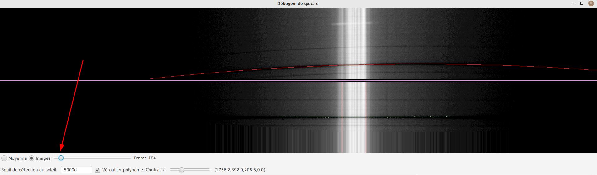
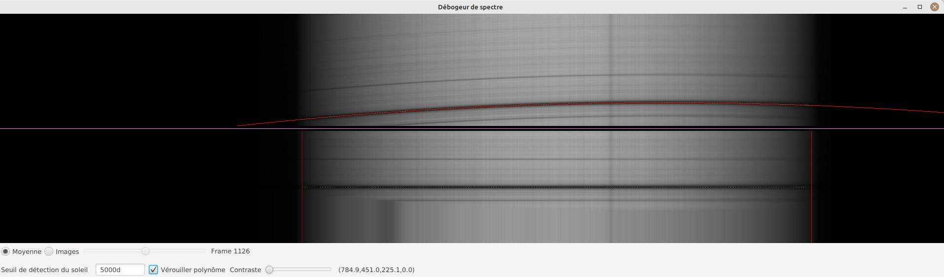
We can now perform measurements: when you are moving the mouse over the image, coordinates are displayed:

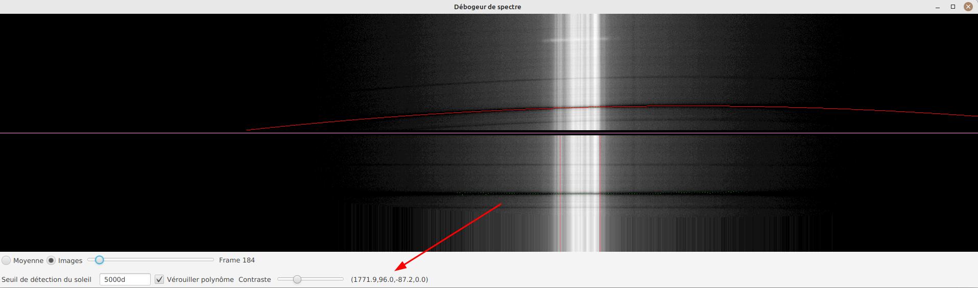
The first 2 numbers are the (x,y) coordinates of the point below the cursor. The 3rd one is the one we’re interested in: it’s the pixel shift between the cursor position and the detected spectral line (in red). The 4th number will let us increase our accuracy by computing an average value from samples.

To add a sample, find a point on the helium line then click on it while holding the CTRL key. You can add as many sample points as you wish.

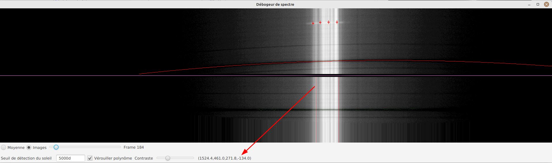
The 4th number is the average of distances and should be a good value to use in your ImageMath scripts. In this example we deduce that the pixel shift is -134.

Optimal exposure calculator

In the "tools" menu, you will find the optimal exposure calculator. This calculator will determine the optimal exposure time, in order to achieve a perfectly circular sun disk and avoid undersampling.

Enter the following parameters:

the camera pixel size (in microns) and the binning
the focal length of your instrument
the scan speed (a multiple of sideral speed, e.g 2, 4, 8, …)
the declination of the sun at the moment of the observation

The software will then automatically compute the optimal exposure time in milliseconds.

Acknowledgements

Christian Buil for designing Sol’Ex and leading the community with great expertise
Valérie Desnoux for her remarkable work on INTI
Jean-François Pittet for his bug reports, test videos, and geometric correction formulas
Sylvain Weiller for his intensive beta-testing, valuable feedback, and processing ideas