JSol’Ex

JSol’Ex is a solar images processing software for Christian Buil’s Sol’Ex. It is capable of processing SER files captured with this instrument in order to produce images of the solar disk, in a similar way to what INTI from Valérie Desnoux is doing. It is primarily designed to process images for Sol’Ex, but it might work properly for other kinds of spectroheliographs.

JSol’Ex is free software published under the Apache 2 software license. It is written in en Java and provided for free without any warranty.

Note to US citizen and far right supporters

If you support Trump or any other party close to the far right, I ask you not to use this software.

My values are fundamentally opposed to those of these parties, and I do not wish for my work, which I have developed during evenings and weekends, and despite it being open source, to be used by people who support these nauseating ideas.

Solidarity, openness to others, ecology, fight against discrimination and inequality, respect for all religions, genders, and sexual orientations are the values that drive me. I do not accept that my work be used by people who are responsible for suffering and exclusion. If you do, I kindly ask you to review your choices and turn to more positive values, where your well-being does not come from the rejection of others.

Downloads

Click on the button corresponding to your OS below:

JSol’Ex (Windows) JSol’Ex (Linux) JSol’Ex (Mac ARM64) JSol’Ex (Mac Intel)

JSol’Ex can also be downloaded or built from source from this page. Installaters are available for Linux, Windows and MacOS.

Alternatively, you may run JSol’Ex by checking out the sources and running the following command:

./gradlew jsolex:run

Community

You can join the JSol’Ex community on the Discord server to share your images, discuss JSol’Ex or ask for help.

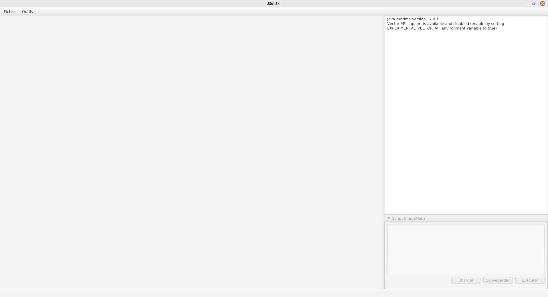
Processing a video file

JSol’Ex only supports SER files, please make sure to configure your capture software to use this format. The main window looks like this:

In the "File" menu, choose "Open SER File" and select a file. The following popup should open:

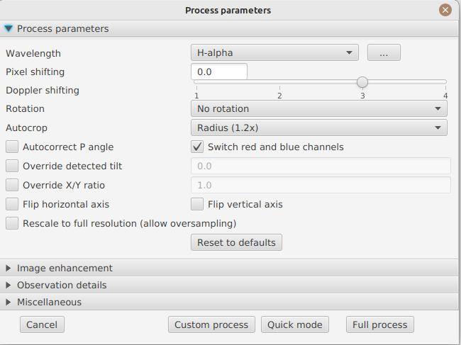
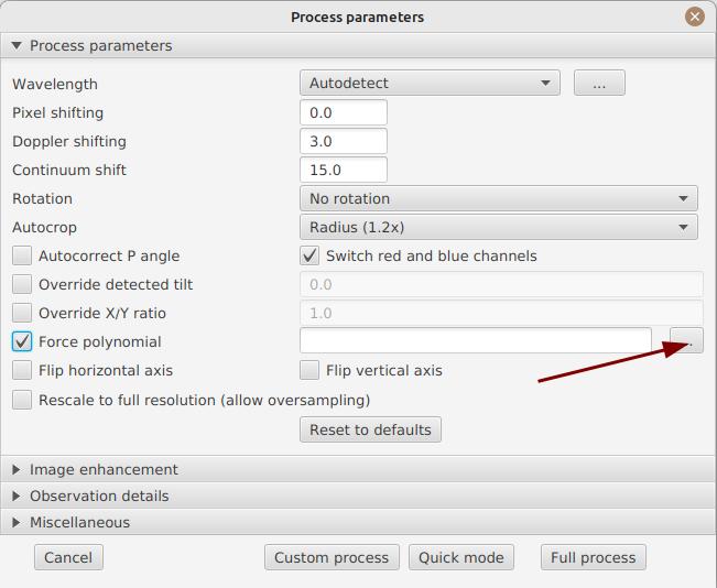
This window is the main entry point for the process parameters. You can specify:

the observation bandwidth: while it’s not mandatory to select that field, doing so will enable automatic colorization of the images. Should your observation bandwidth not be available in the list, you can add more by clicking on the "…" button.
Pixel shift : by default, the software will identify the darkest line in the image and model it as a second order polynomial. Then the image is reconstructed by picking the center of the line, which corresponds to a shift of 0. By using a different shift value, you can produce an image which is "off center", for example to produce images of the solar continuum or to select a different wavelength which isn’t the darkest, such as when observing in helium for example
the Doppler shift is only used when you are observing in h-alpha. JSol’Ex will produce a couple more images shifted in one direction and the other in order to produce a Doppler image. By default, a shift of 3 pixels is used but you can override that parameter.
Rotation : allows performing a left or right rotation (90 degrees) of the images. This can be useful for scans performed in declination, to fix the orientation. This parameter doesn’t affect images produced with ImageMath.
Autocrop : allows automatic cropping of images after geometric transformation. There are multiple modes:
- Off: no autocrop (this is the default)
- Original width: the image will be cropped to a square which width corresponds to the width of the original SER file. Ideal for full solar disks.
- Radius (x…) : the image will be cropped or rescaled to a factor of the determined solar radius. This can be useful for example with truncated disks, if you want to "see" where it would be positioned.
Autocorrect P angle: when checked, the solar angle P will be computed from the observation date (available in the SER file). The generated images will be automatically corrected so that the North is at the top. This parameter will not affect images generated via ImageMath, which need to perform their own correction.
Force tilt: the software is fitting an ellipse around the solar disk which is reconstructed, and uses that information to perform geometric correction. It is possible that the tilt detection is wrong, in which case you can force a value.
Force X/Y ratio: similarly, the X/Y ratio which is detected may be inaccurrate, in which case you can force it to a particular value.
Force polynomial: this lets you override the detected spectral line, if for some reason it is not detected correctly. See the section about forcing the polynomial for more information.
Horizontal and vertical inversion let you mirror the image so that you match the North and East as expected in the output images.
Rescale to full resolution: can be used if your video is oversampled, which typically happens if you are scanning at lower rates (e.g sideral) and that you want to resize the generated image to its full resolution.

Enabling full resolution can lead in significantly larger images and very high memory pressure. It is not recommended to enable this flag.

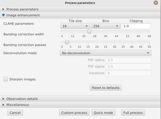
Image enhancement

This section lets you configure the transformations which will be applied to images in order to improve their aesthetic aspect.

CLAHE parameters : allows configuring the CLAHE contrast improvement algorithm. It is possible to configure the size of the tiles used to compute histograms, the histogram resolution and the clipping factor.

Next come the banding correction parameters, which allow to correct transversal bands which can appear on images, for example because of dust on the slit.

Banding correction width: this is the width of the bands which are used in the transversallium correction algorithm. Bands are used to compute the average brightness of pixels in the band, then lines are corrected according the band they belong to.
Banding correction passes: the more passes you’ll apply, the more lines should be corrected, at the cost of lower contrast images

Another section lets you configure image deconvolution. By default, no deconvolution is applied, but you can choose the deconvolution algorithm and its parameters.

For the Richardson-Lucy deconvolution, you can choose the size of the synthetic PSF, the sigma factor and the number of iterations.

Finally, you can choose to apply a detail enhancement filter at the end of the processing by checking the "sharpen images" box.

Experimental

The artificial flat correction allows to correct a possible vignetting. It computes a model from the disk pixels. The pixels considered are those whose value is between a low and a high percentile. For example, if you enter 0.1 and 0.9, the pixels whose value is between the 10th and 90th percentile will be used to compute the model. Finally, a polynomial of the specified order is adjusted on the model values to correct the image.

Observation parameters

Observation parameters are used to insert metadata into FITS files. As of now, we do not recommend to publish images produced using JSol’Ex to the BASS2000 database because the FITS header that this software uses are not validated against what the database expects.

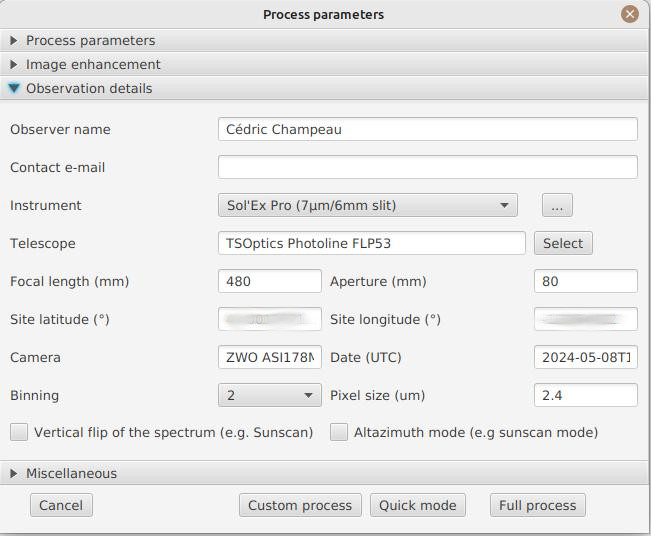
Here are the fields available in JSol’Ex:

Observer : the person who made the observation
Email : the email address of the person who made the observation
Instrument : pre-filled to "Sol’Ex"
Telescope : your telescope or refractor used with the Sol’Ex instrument
Focal length and aperture of the telescope
Latitude and longitude of the observation site
Camera
Date : pre-filled with information from the SER file, expressed in the UTC timezone
Binning : the binning of pixels when the video was recorded
Pixel size : the size of the camera pixels in microns
Vertical flip of the spectrum : normally, the spectrum should have the blue wing at the top and the red wing at the bottom. If it’s the opposite, you can check this box. This is typically the case if you are using a Sunscan.
Alt-Az mode : check this box if you are not using an equatorial mount but an alt-az mount.

Alt-Az mode and image orientation correctness

It is important to understand that JSol’Ex is not capable of determining if an image is flipped vertically or horizontally, but it can compute the solar angle P from the observation date. However, the orientation grid that is generated will only be correct if you are using an equatorial mount. If you are using an alt-az mount, then the orientation grid will be incorrect, as well as the position of the labels of detected active regions. In order to fix this, you must check the "Alt-Az" box and enter your observation site coordinates: JSol’Ex will then compute the parallactic angle and perform correction automatically, resulting in a well oriented image.

Other parameters

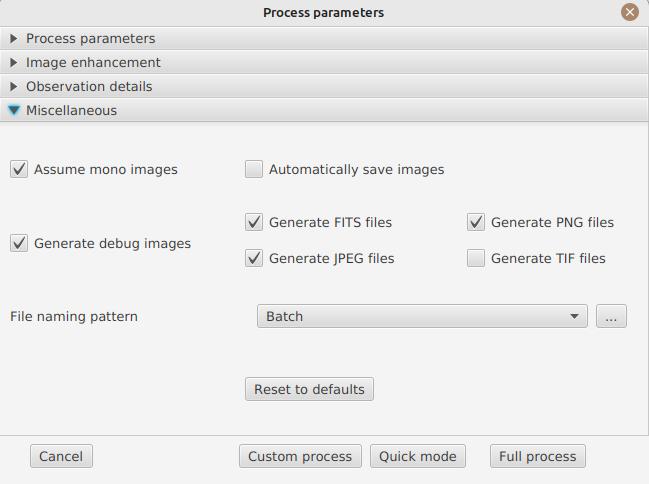
Assume mono video : when checked, JSol’Ex will not try to perform demosaicing of the video, by assuming it’s a mono one. This can considerably speedup processing, and because most videos for Sol’Ex will be mono, it is better to leave this checked.
Automatically save images : if checked, all images which are generated by the software will be saved to disk immediately. If unchecked, then it’s your responsibility to save them by clicking on the "save" button of each image tab.
Generate debug images: when checked, additional images will be generated to highlight edge detection, tilt detection and average image. These can be useful to figure out what when wrong when the software doesn’t produce the expected results.
Generate FITS files : in addition to PNG files, will also generate FITS files.

Force polynomial

JSol’Ex performs detection of the spectral line by looking for the darkest line in the image, then fitting a 3rd order polynomial to it. Sometimes, detection may be incorrect, in which case you can force a polynomial to be used.

In order to do this, click on the "force polynomial" button, which will let you enter the polynomial coefficients.

The format of the polynomial is a list of 4 numbers between curly braces, separated by commas, for example: {1.3414109042116584E-10,3.889927699830093E-5,-0.056529799336687114,35.76051527062038}.

The easiest way to get the polynomial coefficients is to click on the "…" button, which will open a window with the average image and the detected spectral line :

You can then press "CTRL" then click on the line to add measurement points: a red cross will be added for each point. When you have enough points, click on the "Compute polynomial" button, which will fit a 3rd order polynomial to the points and automatically fill the "force polynomial" field in the process parameters:

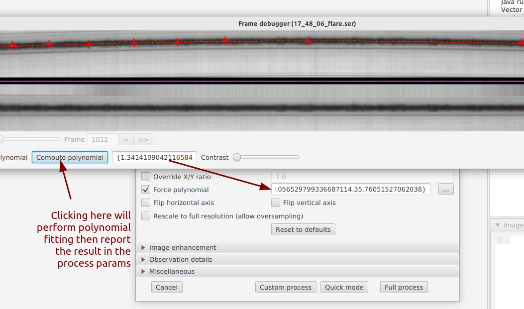
You can then close the popup and start processing.

File naming patterns

By default, JSol’Ex will output the generated images in a subfolder which name matches the name of the SER file (without extension). Then each kind of images is stored in a subdirectory of that folder (e.g raw, debug, processed, …). If that naming convention doesn’t suit you, you can create your own naming patterns, by clicking the "…" dots:

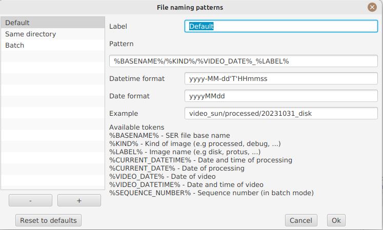
A naming pattern consists of a label, but more importantly a pattern consisting of tokens delimited by the % character.

Please find below the list of available tokens:

%BASENAME% is the SER file base name, that is to say the name without extension
%KIND% is the kind of images (raw, debug, processed, …)
%LABEL% is the label of the produced images, e.g recon, protus
%CURRENT_DATETIME% is the date and time of processing
%CURRENT_DATE% is the date of processing
%VIDEO_DATETIME% is the date and time of the video
%VIDEO_DATE% is the date of the video
%SEQUENCE_NUMBER% is the sequence number in case of batch processing (4 digits, eg. 0012)

This for example would be a pattern which puts all generated files in a single folder:

%BASENAME%/%SEQUENCE_NUMBER%_%LABEL%

The "example" field shows you what the generated file names would look like.

Process start

JSol’Ex provides 3 processing modes: quick, full and custom.

The "quick" mode will only produce a couple images: the raw reconstructed one, and a geometry corrected version. It is useful in your initial setup, when you’re still trying to figure out the tilt or exposure, for example. It is recommended to combine this mode with not saving images automatically, so that you don’t fill your disk with images that you will never use.
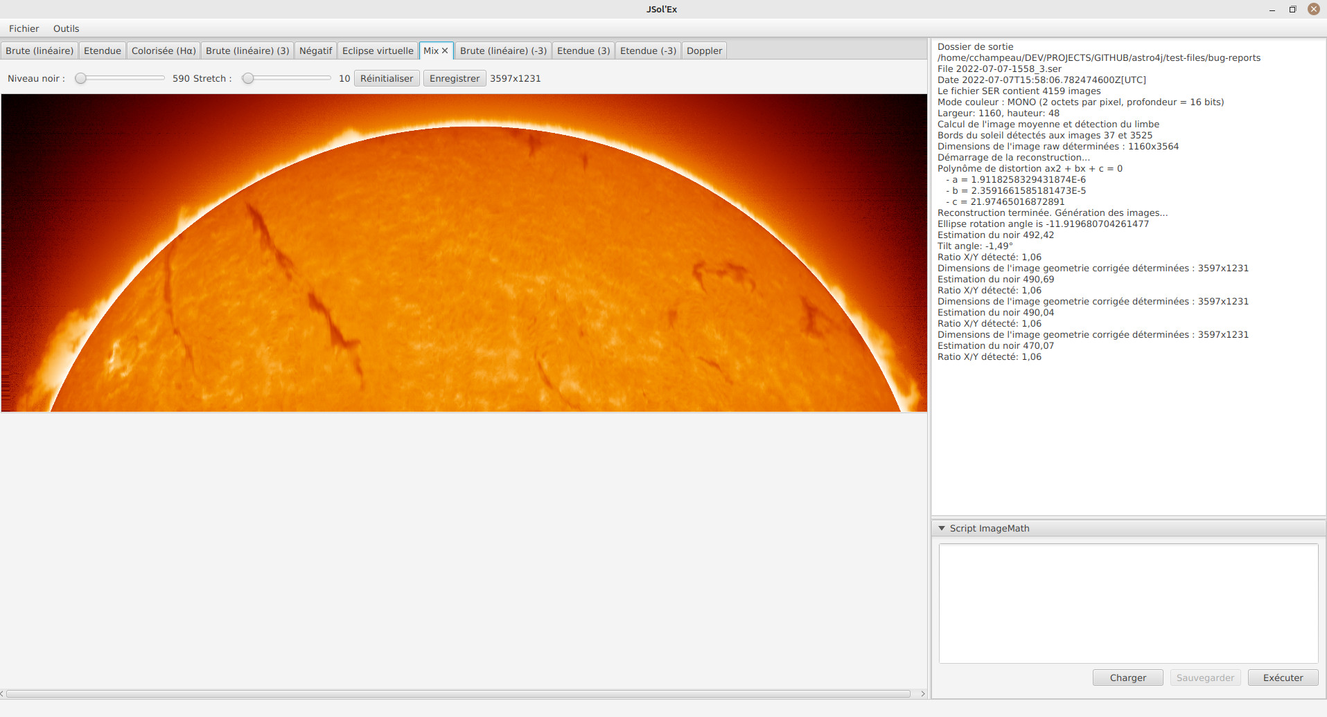
The "full" mode will generate all images that JSol’Ex can automatically produce:
the raw, reconstructed image
a geometry corrected and color-stretched version
a colorized image, if the bandwidth you have selected provides the required parameters
a negative image version
a virtual eclipse, to simulate a coronagraph
a mixed image combining the colorized version with the virtual eclipse
a Doppler image
the "custom" mode will let you precisely pick which images you want to generate. It even provides a more advanced mode letting you script generated images, allowing the generation of images which weren’t designed initially (see the section about custom images).

Image display

Once images are generated, they appear one after each other in tabs. These tabs provide you with the ability to tweak the contrast of images and save them, typically when you unchecked the automatic save option.

It is possible to zoom into the images by using the mouse wheel. In addition, right-clicking the image will let you open it into your file explorer or in a separate window.

Watching a directory for changes

When trying to find the ideal focus, it can be useful to process video files quickly until we obtain a satisfying result. JSol’Ex offers an easy way to do this, by watching the changes in a directory : new videos which are saved in that directory will immediately be processed.

To do this, in the file menu, choose "Watch directory" then select the directory where your SER files will be recorded (e.g the output directory of SharpCap).

JSol’Ex will switch to watch mode, which you can interrupt by clicking the button which appeared in the bottom left of the interface.

Now, open your capture software and record a new video. Once it’s done, switch to JSol’Ex : it will open the process parameters configuration window. Select your processing parameters then start the processing.

Once you have the result, switch back to your capture software and acquire a new video. Once its done, switch back to JSol’Ex: this time, the process parameters window won’t open, because it’s going to reuse the parameters from the first video, allowing to process new videos very quickly!

Make sure that when you switch from your capture software to JSol’Ex that the recording is finished. If not, processing can start on an incomplete file and fail.

Once you’re happy with the result, click on the "Stop watching" button on the bottom left.

You can combine the watch mode with opening an image in a new window (by right-clicking on an image, you can open it in a new window). When a new SER file will be processed, the corresponding image will automatically replace the one in the external window. This can be useful in demonstrations, if you have for example a separate monitor where you would only show the result of processing.

Customization of generated images

When you click the "custom" mode instead of the quick or full ones, JSol’Ex provides you with an interface which will let you declare exactly what should be output.

There are 2 modes available: the simple one and the ImageMath one.

In the simple one, you can pick which images to generate by clicking the right boxes. It is also possible to ask for the creation, in parallel, of images at different pixel shifts.

For example, should you want to generate images from the continuum to the observed ray, you can enter -10;-9;-8;-7;-6;-5;-4;-3;-2;-1;0;1;2;3;4;5;6;7;8;9;10 which will have the consequence of generating 21 distinct images ranging from shift -10 to +10. This can be particularly useful if you want, for example, to generate an animation.

It’s worth noting that if you check some images like "Doppler", some pixel shifts will be automatically added to the list (e.g -3 and +3).

If this isn’t good enough for you, you can go even more advanced by enabling the "ImageMath" mode which is extremely powerful while relatively simple to grasp.

Trimming SER files

It is not unsual to have SER files which contain a lot of empty frames at the beginning or at the end, because of how we usually capture videos: we start the capture, then we wait for the mount to stabilize, then we stop the capture. In addition, our cropping window may be a bit too large for what we actually want to study.

As a consequence, SER files stored on disk are usually significantly larger than what they need to be. Since JSol’Ex 2.10, a new option is available at the end of the processing of a file. You can click on the "Trim SER file" button on the top right corner of the interface, which will open a new window:

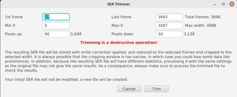
This window is pre-filled with parameters which are deduced from the processed file. In particular, the start and end frames, as well as the mininum and maximum X values (width) are automatically determined from the detection of the solar disk in the video. A reasonable margin of 10% is added, which means that sometimes, the first and last frame may actually correspond to the full video if you actually have video where the sun appears quickly in the field of view.

The "pixels up" and "pixels down" parameters correspond to how many pixels you want to keep in the target SER file. Again these are automatically determined from the correction of the "smile" (the curvature of the spectral line), but it may be particularly interesting to reduce, since it will have a large impact on the size of the file. However, reducing the number of pixels up/down will remove information from the video (you won’t be able to compute images with larger pixel shifts), so always be careful not to reduce it too much.

Once you’re happy with the parameters, click on "Trim" and a new SER file will be created in the same directory as the original one, with the suffix _trimmed.

It’s worth noting that the trimmed video will also have the smile correction applied, which means that the spectral line will be centered in the video and that each line will be perfectly horizontal. This information is used by JSol’Ex in case you decide to process the trimmed video, so that you don’t have to recompute the smile correction.

It is important to understand that trimming is a destrutive operation: when you reduce the number of frames or the min x/max x values, then you are potentially truncating the solar disk or features like prominences. If you are selecting too low pixel up/down values, then you are reducing the bandwidth of observation, which means for example that you may not be able to generate a continuum image anymore. In both cases, the result of processing the trimmed video will be different from the original one.

Here’s an example of a video:

And the result after trimming:

ImageMath : images generation scripts

Introduction to ImageMath

The "ImageMath" mode is a mode which will let you declare which images to generate by writing small scripts. It relies on a simple script language designed specifically for generating Sol’Ex images.

Let’s illustrate this by going back to our previous example, where you wanted to generate images in the [-10;10] pixel shift range. In the "simple" mode, you had to manually enter all pixel shifts, which can be a little cumbersome. In the "ImageMath" mode, we have a language which will let us to this with a single instruction.

First, select the ImageMath mode in the select box and click on "Open ImageMath". The following interface show up:

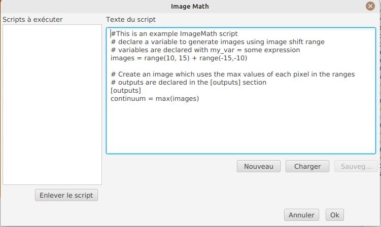
On the left side, "Scripts to execute", you will find the list of all scripts which will be applied in your session.

This is really the list of scripts which are applied in that session, not the list of available scripts! Click on the "remove" button to remove scripts from execution in the session.

Scripts must be saved on your local disk and can be shared with other users. Their contents is editable in the rightmost part of the interface.

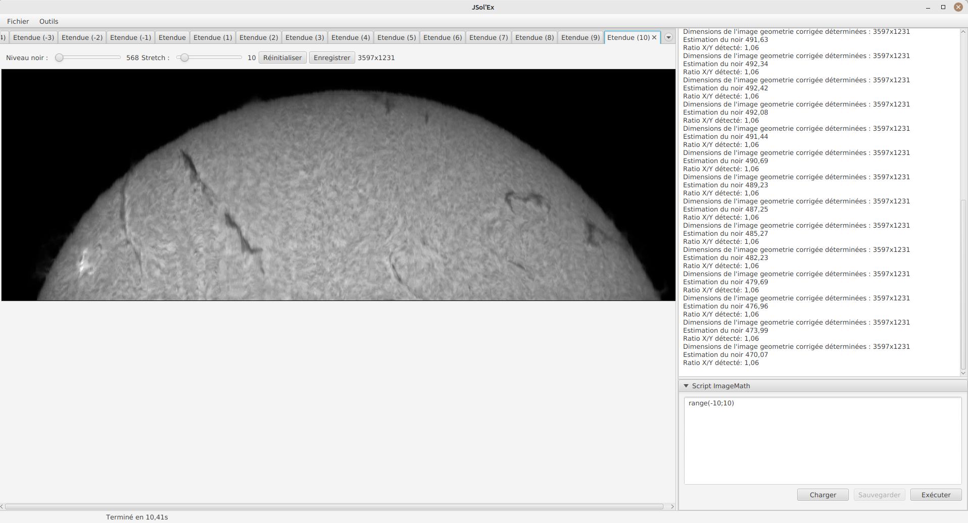
Start with removing the contents of the sample script and replace it with:

range(-10;10)

Then click on "Save". Select a destination file and proceed: the script is now added to the list on the left, as being executed in this session.

Click on "Ok" to close ImageMath and only keep the "geometry corrected (stretched)" images. Click on "Ok" to start processing, you will now have the 21 required images generated:

Functions available in ImageMath

For now we’ve only used one function called range, which let us generate about 20 images, but there are many others available.

Solar Image Reconstruction

IMG

Returns the reconstructed image at the specified pixel offset.

Argument

Required?

Description

Default value

ps

Pixel shift

Examples

img(0)

img(ps: 1)

img(ps: a2px(1)) // 1 Å pixel shift

RANGE

Returns the reconstructed image at the pixel offsets represented by the interval.

Argument

Required?

Description

Default value

from

to

End of the interval (inclusive)

step

Step of the interval

Examples

range(-1;1)

range(-1;1;0.5))

range(from: -10; to: 10; step: 2)

Math functions

AVG

Computes the average of its arguments. If the arguments are images, the average is computed pixel-wise.

Argument

Required?

Description

Default value

list

Arguments

Examples

avg(range(-1;1))

avg(img(0); img(1))

CONCAT

Concatenates argument lists.

Argument

Required?

Description

Default value

list

Arguments

Examples

concat(list(img(0));range(-1;1))

EXP

Computes an exponential

Argument

Required?

Description

Default value

v

Value

exp

Exponent

Examples

exp(img(0); 1.5)

exp(v:img(0), exp: 2)

exp(2, 3)

exp(v:2, exp: 3)

LOG

Computes a logarithm

Argument

Required?

Description

Default value

v

Value

exp

Exponent

Examples

log(img(0); 1.5)

log(v:img(0), exp: 2)

log(2, 3)

log(v:2, exp: 3)

MAX

Computes the maximum of its arguments. If the arguments are images, the maximum is computed pixel-wise.

Argument

Required?

Description

Default value

list

Arguments

Examples

max(range(-1;1))

max(img(0); img(1))

MEDIAN

Computes the median of its arguments. If the arguments are images, the median is computed pixel-wise.

Argument

Required?

Description

Default value

list

Arguments

Examples

median(range(-1;1))

median(img(0); img(1))

MIN

Computes the minimum of its arguments. If the arguments are images, the minimum is computed pixel-wise.

Argument

Required?

Description

Default value

list

Arguments

Examples

min(range(-1;1))

min(img(0); img(1))

POW

Computes a power

Argument

Required?

Description

Default value

v

Value

exp

Exponent

Examples

pow(img(0); 1.5)

pow(v:img(0), exp: 2)

pow(2, 3)

pow(v:2, exp: 3)

WEIGHTED_AVG

Computes a weighted average of images

Argument

Required?

Description

Default value

images

Images

weights

Weights

Examples

weighted_avg(range(-1;1);list(.5;1;.5))

weighted_avg(images: range(-1;1); weights: list(.5;1;.5)))

Utilities

AR_OVERLAY

Generates an overlay of the detected active regions. This feature will only work if active region image generation has been selected.

Argument

Required?

Description

Default value

img

Image(s)

labels

0 : do not display 1 : display the regions and the labels 2 : display only the labels

Examples

ar_overlay(continuum())

ar_overlay(img: img(0); labels: 2)

CHOOSE_FILE

Opens a dialog box to choose an image file.

Argument

Required?

Description

Default value

id

An ID for the file chooser. The next time the function is called with the same ID, the directory where the file chooser was opened will be used as the starting point.

message

Title of the dialog box

Examples

choose_file("my_id", "Choose a file")

choose_file(id: "my_id", title: "Choose a file")

CHOOSE_FILES

Opens a dialog box to choose multiple image files.

Argument

Required?

Description

Default value

id

An ID for the file chooser. The next time the function is called with the same ID, the directory where the file chooser was opened will be used as the starting point.

message

Title of the dialog box

Examples

choose_files("my_id", "Choose a file")

choose_files(id: "my_id", title: "Choose a file")

ELLIPSE_FIT

Triggers a new detection of the shape of the solar disk.

Argument

Required?

Description

Default value

img

Image(s)

Examples

ellipse_fit(img(0))

ellipse_fit(img:range(0;1))

FILTER

The filter function can be used on a list of images to keep these which match a particular criteria. This can be particularly useful in batch mode. For example, you may want to perform a vertical and horizontal flip to images after a certain time, because of meridian flip.

Argument

Required?

Description

Default value

img

List of images to filter.

subject

Sbject of the filter (file-name, dir-name, pixel-shift, time or datetime).

function

Operator to apply to filter the images.

value

Value for comparison

Subject Description Available operators Example

file-name

The name of the SER file

=, `

=, `contains, starts_with, ends_with

filter(images, "file-name", "contains", "2021-06-01")

dir-name

The name of the directory which contains the SER file

=, `

=, `contains, starts_with, ends_with

filter(images, "dir-name", "contains", "2021-06-01")

pixel-shift

The pixel shift of the image

=, `

=, `>, <, >=, ⇐

filter(images, "pixel-shift", ">", 0)

time

The time of the acquisition (compared in UTC)

=, `

=, `>, <, >=, ⇐

filter(images, "time", ">", "12:00:00")

datetime

The date and time of the acquisition (compared in UTC)

=, `

=, `>, <, >=, ⇐

Examples

filter(images, "file-name", "contains", "2021-06-01")

filter(img: images, subject:"file-name", function:"contains", value:"2021-06-01")

filter(images, "dir-name", "contains", "2021-06-01")

filter(imgimages, subject:"dir-name", function:"contains", value:"2021-06-01")

filter(images, "pixel-shift", ">", 0)

filter(images, "time", ">", "12:00:00")

filter(images, "datetime", ">", "2021-06-01 12:00:00")

GET_AT

Returns the value of an element in a list at the specified position.

Argument

Required?

Description

Default value

list

List

index

Index

Examples

get_at(list; 0)

get_at(list: some_list; index: 1)

GET_B

Extracts the blue channel from an image.

Argument

Required?

Description

Default value

img

Image(s)

Examples

get_b(some_image)

get_b(img: some_image)

GET_G

Extracts the green channel from an image.

Argument

Required?

Description

Default value

img

Image(s)

Examples

get_g(some_image)

get_g(img: some_image)

GET_R

Extracts the red channel from an image.

Argument

Required?

Description

Default value

img

Image(s)

Examples

get_r(some_image)

get_r(img: some_image)

LIST

Creates a list from the parameters.

Argument

Required?

Description

Default value

list

List

Examples

list(img(-3), img(3))

list(list: img(-3), img(3))

LOAD

Loads an image from a file.

Argument

Required?

Description

Default value

file

File path

Examples

load('image.fits')

load(file: '/path/to/image.fits')

LOAD_MANY

Loads many images from a directory.

Argument

Required?

Description

Default value

dir

Directory path

pattern

Regular expression to filter files

Examples

load_many("/chemin/vers/dossier")

load_many(dir: "/chemin/vers/dossier", pattern:".*cropped.*")

MONO

Converts a color image to grayscale.

Argument

Required?

Description

Default value

img

Image(s)

Examples

mono(some_image)

mono(img: some_image)

REMOTE_SCRIPTGEN

Experimental, advanced function which is described specifically in this section.

Argument

Required?

Description

Default value

url

URL of the service to invoke

Examples

remote_scriptgen("http://localhost:8080/jsolex/remote")

remote_scriptgen(url: "http://localhost:8080/jsolex/remote")

RGB

Creates an RGB image from three mono images.

Argument

Required?

Description

Default value

r

Red image

g

Green image

b

Blue image

Examples

rgb(img(-1);img(0);img(1))

rgb(r: redWing; g: avg(redWing;blueWing); b: blueWing)

SORT

Sorts a list of images

Argument

Required?

Description

Default value

images

Images

order

Sort order. One of date, shift or file_name, modulated by asc or desc.

shift

Examples

sort(images, 'date')

sort(images, 'date asc')

sort(images: images, order: 'date desc')

VIDEO_DATETIME

Returns the datetime when a video was recorded.

Argument

Required?

Description

Default value

img

Image(s)

format

Date format.

Examples

video_datetime(img(0))

video_datetime(img: img(0), format:"yyyy-MM-dd HH:mm:ss")

WAVELEN

Returns the wavelength of an image.

Argument

Required?

Description

Default value

img

Image(s)

Examples

wavelen(img(0))

wavelen(img: img(0))

WORKDIR

Changes the working directory in which images are loaded by the LOAD and LOAD_MANY functions.

Argument

Required?

Description

Default value

dir

Working directory

Examples

workdir('/path/to/dir')

workdir(dir: '/path/to/dir')

Image Enhancement

ADJUST_CONTRAST

Applies simple contrast adjustment by clipping values under the minimal value or above the maximal value.

Argument

Required?

Description

Default value

img

Image(s)

min

Minimum value

max

Maximum value

Examples

adjust_contrast(img: img(0), min: 10, max: 200)

adjust_contrast(img(0), 10, 200)

ADJUST_GAMMA

Applies a gamma correction to an image.

Argument

Required?

Description

Default value

img

Image(s)

gamma

Gamma

Examples

adjust_gamma(img: img(0), gamma: 2.2)

adjust_gamma(img(0), 1.5)

ASINH_STRETCH

Applies the inverse arcsin hyperbolic transformation to increase contrast.

Argument

Required?

Description

Default value

img

Image(s)

bp

Black point

stretch

Stretch factor

Examples

asinh_stretch(img: img(0), bp: 500, stretch: 2.5)

asinh_stretch(img(0), 0, 10)

AUTO_CONTRAST

This function is a contrast enhancement function specifically designed for spectroheliograph images.

Argument

Required?

Description

Default value

img

Image(s)

gamma

Gamma

bg

Background correction aggressiveness between 0 and 1. 1 = no correction, 0 = maximum correction.

Examples

auto_contrast(img: img(0), gamma: 1.5)

auto_contrast(img(0), 1.5)

BLUR

Applies a Gaussian blur to an image.

Argument

Required?

Description

Default value

img

Image(s)

kernel

Kernel size

Examples

blur(img(0))

blur(img(0), 7)

blur(img: img(0), kernel:7)

CLAHE

Applies CLAHE (Contrast Limited Adaptive Histogram Equalization) transformation to an image.

Argument

Required?

Description

Default value

img

Image(s)

ts

Tile size

bins

Bin count

clip

Clip limit

Examples

clahe(img: img(0), ts: 16, bins: 128, clip: 1.1)

clahe(img(0), 16, 128, 1.1)

COLORIZE

Applies a colorization to an image using a color profile related to the wavelength.

Argument

Required?

Description

Default value

img

Image(s)

profile

Color profile (see spectral lines editor)

Examples

colorize(img: img(0), profile: "H-alpha")

colorize(range(-1, 1), "Calcium (K)")

COLORIZE2

Applies a colorization to an image using curve modeling. The curves are defined by 2 control points: the input value and the output value.

Argument

Required?

Description

Default value

img

Image(s)

rIn

Input value for red (0-255)

rOut

Output value for red (0-255)

gIn

Input value for green (0-255)

gOut

Output value for green (0-255)

bIn

Input value for blue (0-255)

bOut

Output value for blue (0-255)

Examples

colorize(img: img(0), profile: "H-alpha")

colorize(range(-1, 1), "Calcium (K)")

CURVE_TRANSFORM

Applies a curve transformation to an image. The transformation interpolates a polynomial of degree 2 passing through three points: the origin point (0,0), the curve point (in, out), and the extreme point (255,255).

Argument

Required?

Description

Default value

img

Image(s)

in

Input value of the curve (0-255)

out

Output value of the curve (0-255)

Examples

curve_transform(img(0), 100, 120)

curve_transform(img: img(0), in:50, out: 200)

DISK_FILL

Fills the detected solar disk with a given value (default is the value of the detected black point).

Argument

Required?

Description

Default value

img

Image(s)

fill

Fill value

detected black point value

Examples

disk_fill(img(0))

disk_fill(img: img(0), fill: 200)

DISK_MASK

Creates a mask of the solar disk, where pixels inside the disk will have the value 1, against 0 for those outside the disk. It is possible to invert (0 inside, 1 outside) by passing 1 as the 2nd parameter of the function.

Argument

Required?

Description

Default value

img

Image(s)

invert

Inversion of the mask (1 means value 0 inside, 1 outside)

Examples

disk_mask(img(0))

disk_mask(img: img(0), invert: 1)

EQUALIZE

Equalizes the histogram of the images in parameter so that they all have about the same brightness.

Argument

Required?

Description

Default value

list

List of images to equalize.

Examples

equalize(range(-1;1))

equalize(list: some_images)

FIX_BANDING

Applies a banding correction to the image

Argument

Required?

Description

Default value

img

Image(s)

bs

Band size

passes

Number of passes

Examples

fix_banding(img(0), 64, 3)

fix_banding(img: img(0), bs: 48, passes: 10)

FIX_GEOMETRY

Applies geometric correction to the image based on the calculated ellipse

Argument

Required?

Description

Default value

img

Image(s)

Examples

fix_geometry(img(0))

fix_geometry(img: img(0))

FLAT_CORRECTION

Computes an artificial flat field image to correct the image then applies the correction.

Argument

Required?

Description

Default value

img

Image(s)

lo

Low percentile value

0.1

hi

High percentile value

0.95

order

Polynomial order

[NOTE] .Experimental ==== The artificial flat correction allows to correct a possible vignetting. It computes a model from the disk pixels. The pixels considered are those whose value is between a low and a high percentile. For example, if you enter 0.1 and 0.9, the pixels whose value is between the 10th and 90th percentile will be used to compute the model. Finally, a polynomial of the specified order is adjusted on the model values to correct the image. ====

Examples

flat_correction(img(0))

flat_correction(img: img(0), order: 3)

INVERT

Inverts the colors of an image.

Argument

Required?

Description

Default value

img

Image(s)

Examples

invert(img(0))

invert(img: img(0))

LINEAR_STRETCH

Stretches the histogram of an image to occupy the entire range of possible values. This function can also be used to compress the values of an image into the range of possible values (for example after an exponential calculation).

Argument

Required?

Description

Default value

img

Image(s)

lo

Minimum value of the histogram to stretch.

hi

Maximum value of the histogram to stretch.

65535

Examples

linear_stretch(img(0))

linear_stretch(img(0), 10000, 48000)

linear_stretch(img: img(0), hi: 48000)

RL_DECON

Applies the Richardson-Lucy deconvolution algorithm to the image.

Argument

Required?

Description

Default value

img

Image(s)

radius

Gaussian radius

2.5

sigma

Sigma

2.5

iterations

Number of iterations

Examples

rl_decon(img(0))

SATURATE

Saturates the colors of an image.

Argument

Required?

Description

Default value

img

Image(s)

factor

Saturation

Examples

saturate(img(0);1.5)

saturate(img: img(0); factor: 1.5)

SHARPEN

Applies a sharpening filter to an image.

Argument

Required?

Description

Default value

img

Image(s)

kernel

Kernel size

Examples

sharpen(img(0))

sharpen(img(0), 7)

sharpen(img: img(0), kernel:7)

Cropping

AUTOCROP

Automatically crops an image around the solar disk. The dimensions of the cropping area are determined by the ellipse but also by the dimensions of the image. It is better to use the autocrop2 function which guarantees a centered and square crop.

Argument

Required?

Description

Default value

img

Image(s)

Examples

autocrop(img: img(0))

autocrop(img(0))

AUTOCROP2

Crops an image to a centered and square area around the solar disk.

Argument

Required?

Description

Default value

img

Image(s)

factor

The width of the image will be the diameter of the solar disk multiplied by this factor.

1.1

rounding

The width of the image will be rounded to this multiple. Must be a multiple of 2.

Examples

autocrop2(img: img(0))

autocrop2(img(0))

CROP

Crops an image to the specified coordinates and dimensions.

Argument

Required?

Description

Default value

img

Image(s)

left

X coordinate of the top left corner of the cropping area.

top

Y coordinate of the top left corner of the cropping area.

width

Width of the cropping area.

height

Height of the cropping area.

Examples

crop(img(0), 10, 20, 100, 200)

crop(img: img(0), left: 10, top: 20, width: 100, height: 200)

CROP_AR

Generates a list of images corresponding to the detected sunspots.

Argument

Required?

Description

Default value

img

Image(s)

ms

Minimum size of the spot.

margin

Margin around the spot (in %).

Examples

crop_ar(continuum))

crop_ar(img:img(0), margin: 15)

CROP_RECT

Reduces the image to the specified dimensions, ensuring that the center of the solar disk will be at the center of the image. There is no scaling: if the solar disk does not fit within the target dimensions, it will be cropped.

Argument

Required?

Description

Default value

img

Image(s)

width

Width of the cropping area.

height

Height of the cropping area.

Examples

crop_rect(img(0), 1024, 1024)

crop_rect(img: img(0), width: 200, height: 200)

Background Extraction

BG_MODEL

Creates a BACKGROUND model from an image, which can be used to subtract the BACKGROUND from the original image.

Argument

Required?

Description

Default value

img

Image(s)

order

Polynomial order. A value higher than 3 is not recommended.

sigma

Number of sigmas for sample selection.

2.5

Examples

bg_model(img(0); 2.5; 3)

bg_model(img: img(0); sigma: 3)

NEUTRALIZE_BG

This is a function similar to remove_bg that uses a polynomial modeling of the background to remove gradients. This function can be used on images without ellipse information (solar disk).

Argument

Required?

Description

Default value

img

Image(s)

iterations

Number of iterations of the algorithm.

Examples

neutralize_bg(some_image)

neutralize_bg(img: img(0), iterations: 5)

REMOVE_BG

Performs background removal on an image. This can be used when the contrast is very low (e.g in helium processing) and that stretching the image also stretches the background. This process computes the average value of pixels outside the disk, then uses that to perform an adaptative suppression depending on the distance from the limb, in order to preserve light structures around the limb.

Argument

Required?

Description

Default value

img

Image(s)

tolerance

Tolerance

0.9

Examples

remove_bg(some_image)

remove_bg(img: img(0), tolerance: .5)

Rotation and Rescaling

HFLIP

Flips an image horizontally.

Argument

Required?

Description

Default value

img

Image(s)

Examples

hflip(some_image)

hflip(img: img(0))

RADIUS_RESCALE

Relative scaling method which can facilitate mosaic composition. It will therefore most likely be used in batch mode. It allows rescaling a set of images so that they all have the same solar disk radius (in pixels). In order to do so, it will perform an ellipse regression against each image to compute their solar disk, then will rescale all images to match the radius of the largest one.

Argument

Required?

Description

Default value

images

Image(s)

Examples

radius_rescale(some_image)

radius_rescale(images: my_list)

RESCALE_ABS

Rescales an image to the specified absolute dimensions.

Argument

Required?

Description

Default value

img

Image(s)

width

Width of the image

height

Height of the image

Examples

rescale_abs(img(0), 100, 100)

rescale_abs(img: img(0), width: 100, height: 100)

RESCALE_REL

Rescales an image by applying a rescaling factor.

Argument

Required?

Description

Default value

img

Image(s)

sx

Horizontal rescaling factor

sy

Vertical rescaling factor

Examples

rescale_rel(img(0), .5, .5)

rescale_rel(img: img(0), sx: 0.5, sy: 0.5)

ROTATE_DEG

Applies a rotation to an image, in degrees.

Argument

Required?

Description

Default value

img

Image(s)

angle

Angle

bp

Fill value for pixels outside of the image.

resize

Resize the image to fit the rotation.

Examples

rotate_deg(img(0); 30)

rotate_deg(img: img(0); angle: 30)

ROTATE_LEFT

Applies a left rotation to an image

Argument

Required?

Description

Default value

img

Image(s)

Examples

rotate_left(img(0))

rotate_left(img: img(0))

ROTATE_RAD

Applies a rotation to an image, in radians.

Argument

Required?

Description

Default value

img

Image(s)

angle

Angle

bp

Fill value for pixels outside of the image.

resize

Resize the image to fit the rotation.

Examples

rotate_rad(img(0); 2.1)

rotate_rad(img: img(0); angle: 2.1)

ROTATE_RIGHT

Applies a right rotation to an image

Argument

Required?

Description

Default value

img

Image(s)

Examples

rotate_right(img(0))

rotate_right(img: img(0))

VFLIP

Flips an image vertically.

Argument

Required?

Description

Default value

img

Image(s)

Examples

vflip(some_image)

vflip(img: img(0))

Analysis

A2PX

Computes the number of pixels corresponding to a distance in Angstroms. The distance is determined by calculating the dispersion, which will only be correct if you have correctly specified the pixel size of the camera, as well as your spectroheliograph.

Argument

Required?

Description

Default value

a

Angstroms

ref

Reference wavelength in Angstroms

Examples

a2px(1.2)

a2px(a: 1.2, ref: 6328)

CONTINUUM

Generates a continuum image around the studied line. This function differs from the classic continuum image in that it is not a single image calculated by the difference of fixed pixels of 15 pixels, but an image calculated from the median of a set of images.

Argument

Required?

Description

Default value

Examples

continuum()

FIND_SHIFT

Computes a pixel offset relative to the detected line. The distance is determined by calculating the dispersion, which will only be correct if you have correctly specified the pixel size of the camera, as well as your spectroheliograph.

Argument

Required?

Description

Default value

wl

Wavelength to search for in Angstroms or line name

ref

Reference wavelength in Angstroms

Examples

find_shift(5875.62)

find_shift(wl: 5875.62, ref: 5895.92)

PX2A

Computes the number of angstroms corresponding to a distance in pixels. The distance is determined by calculating the dispersion, which will only be correct if you have correctly specified the pixel size of the camera, as well as your spectroheliograph.

Argument

Required?

Description

Default value

px

pixels

ref

Reference wavelength in Angstroms

Examples

px2a(24)

px2a(px: 24, ref: 6328)

Drawing

DRAW_ARROW

Draws an arrow on the image.

Argument

Required?

Description

Default value

img

Image(s)

x1

Start of the arrow (X coordinate)

y1

Start of the arrow (Y coordinate)

x2

End of the arrow (X coordinate)

y2

End of the arrow (Y coordinate)

thickness

Thickness of the arrow

color

Color of the arrow

Examples

draw_arrow(img(0), 100, 100, 200, 200, 2, "ff0000")

draw_arrow(img:img(0), x1:100, y1:100, x2:200, y2:200, color: "ff0000")

DRAW_CIRCLE

Draws a circle on the image.

Argument

Required?

Description

Default value

img

Image(s)

cx

X coordinate of the center of the circle

cy

Y coordinate of the center of the circle

thickness

Thickness of the arrow

color

Color of the arrow

Examples

draw_circle(img(0), 100, 100, 2)

draw_circle(img:img(0), cx:100, cy:100, color: "ff0000")

DRAW_EARTH

Draws the Earth on the image, to the scale of the solar disk

Argument

Required?

Description

Default value

img

Image(s)

x

X coordinate of the center of the Earth

y

Y coordinate of the center of the Earth

Examples

draw_earth(img(0), 100, 100)

draw_earth(img:img(0), x:100, y:100)

DRAW_GLOBE

Draws a globe whose orientation and diameter correspond to the detected solar parameters.

Argument

Required?

Description

Default value

img

Image(s)

angleP

P angle

angle P

b0

b0 angle

Examples

draw_globe(img(0))

draw_globe(img:img(0), angleP: 0)

DRAW_OBS_DETAILS

Displays observation details on the image

Argument

Required?

Description

Default value

img

Image(s)

x

X coordinate

y

Y coordinate

Examples

draw_obs_details(img(0), 100, 100)

draw_obs_details(img:img(0), x:100, y:100)

DRAW_RECT

Draws a rectangle on the image.

Argument

Required?

Description

Default value

img

Image(s)

left

X coordinate of the top left corner of the rectangle

top

Y coordinate of the top left corner of the rectangle

width

Width of the rectangle

height

Height of the rectangle

thickness

Thickness of the line

color

Color of the line

Examples

draw_rect(img(0), 100, 100, 300, 200)

draw_rect(img:img(0), left:100, top:100, color: "ff0000")

DRAW_SOLAR_PARAMS

Displays solar parameters on the image

Argument

Required?

Description

Default value

img

Image(s)

x

X coordinate

top right

y

Y coordinate

top right

Examples

draw_solar_params(img(0), 100, 100)

draw_solar_params(img:img(0), x:100, y:100)

DRAW_TEXT

Draws text on the image.

Argument

Required?

Description

Default value

img

Image(s)

x

X coordinate

y

Y coordinate

text

Text to write

fs

Font size

auto

color

Color of the arrow

Examples

draw_circle(img(0), 100, 100, 2)

draw_circle(img:img(0), cx:100, cy:100, color: "ff0000")

Animations

ANIM

Creates an animation from a series of images.

Argument

Required?

Description

Default value

images

The list of images

delay

Delay between each frame (in ms)

250

Examples

anim(range(0,10))

anim(images: range(0,10), delay: 100)

TRANSITION

Interpolates images between them. By default, the interpolation is linear and it will create exactly the specified number of images. However, if a unit is specified, then the behavior will be different: the number of steps corresponds to the number of images to create, for a given time unit, for the time elapsed between the two images. For example, if one image was taken at 10:00 and the other at 10:02, and the unit is ipm, that the number of steps is 10, then 20 images will be created. This allows creating smoother transitions when SER files were not recorded at regular intervals.

Argument

Required?

Description

Default value

images

Image(s)

steps

Number of intermediate images to generate.

type

Interpolation type: linear, ease_in, ease_out or ease_in_out.

linear

unit

Interpolation unit: ips (images per second), ipm (images per minute) or iph (images per hour).

Examples

transition(list(img(0), img(1)), 10)

transition(images: my_imges, steps: 10, type: ease_in, unit: ipm)

Stacking and mosaic composition

DEDISTORT

Allows to correct the distortion of an image. It has 2 distinct modes of use. In the first mode, it takes a reference image and an image to correct, as well as 3 optional parameters: the tile size, the sampling, and the sky background value. The returned image will be corrected as closely as possible to the reference image, making it usable for stacking, for example. In the second mode, it takes a list of images to correct and a list of already corrected images, in which case the correction parameters for each image are taken using the same index image in the list of already corrected images. This can be useful, for example, when calculating the distortion at the center of the line (shift 0) and wanting to apply the same corrections to images with different shifts.

Argument

Required?

Description

Default value

ref

Reference image(s)

img

Images to correct.

ts

Tile size

sampling

Sampling. A value of 0.5 for a tile size of 32 pixels means that there will be a sample every 16 pixels.

0.5

threshold

Sky background value.

Examples

crop_rect(img(0), 1024, 1024)

crop_rect(img: img(0), width: 200, height: 200)

MOSAIC

Creates a mosaic of images.

Argument

Required?

Description

Default value

images

Images to be assembled.

ts

Tile size

sampling

Sampling factor

0.25

Examples

mosaic(some_images)

mosaic(images: some_images, ts: 128)

STACK

Stacks multiple images.

Argument

Required?

Description

Default value

images

Images to be stacked.

ts

Tile size

sampling

Sampling factor

0.5

select

Method for selecting the best image. Can be sharpness (sharpest image), average (average of all images), median (median of all images) or eccentricity (roundest sun image). In batch mode, a manual mode is also available.

sharpness

Examples

stack(some_images)

stack(some_images, 64; .5; "eccentricity")

stack(images: some_images, ts: 128, sampling: 0.5, select: "sharpness")

STACK_REF

Selects a reference image for stacking.

Argument

Required?

Description

Default value

images

Images to be stacked.

select

sharpness

Examples

stack_ref(some_images)

stack_ref(some_images, "eccentricity")

stack_Ref(images: some_images, select: "sharpness")

ImageMath scripts

In the previous section, we have seen the building blocks of ImageMath, which permit computation of new images. Scripts go beyond this by combining these into a powerful tool to generate images. As an illustration, let’s look at this script which will let us generate an Helium image. Helium image processing is complicated, because the Helium ray is very dim and the software cannot find it in the image. Therefore, we can use a technique which consists of taking a larger capture window which includes a dark ray, then by determining by how many pixels the helium ray is shifted from that line, we can reconstruct an image. Even so, the work is not finished, since it’s an extremely low contrast ray, so we have to substract the continuum value. Producing such images is quite cumbersome but can be simplified to the extreme with ImageMath:

[params]
# The shifting between the helium line and the detected line (in pixels)
Line=5875.62
HeliumShift=find_shift(Line)
# Banding correction width and number of iterations
BandWidth=25
BandIterations=20
# Contrast adjustment
Gamma=1.5
# Autocrop factor (of diameter)
AutoCropFactor=1.1

## Temporary variables
[tmp]
helium_raw = img(HeliumShift) - continuum()
helium_fixed = fix_banding(helium_raw;BandWidth;BandIterations)
cropped = autocrop2(auto_contrast(helium_fixed;Gamma);AutoCropFactor)

## Let's produce the images now!
[outputs]
helium_mono = cropped
helium_color = colorize(helium_mono, Line)

Our script consists of 3 different sections: [params], [tmp] and [outputs]. The only mandatory section is the [outputs] one: it defines which images we want to have in the end. The name of all other sections is arbitrary, you can create as many sections as you want.

Here, we defined a [params] section which highlights which parameters we want users to be able to tweak for their needs. This is where we find the value of our helium ray pixel shift (HeliumShift=find_line(Line)) which is computed from the Line=5875.62 variable declaration.

A variable can only contain ASCII characters, digits (except for the 1st character) or the _ character. For example, myVariable, MyVariable or MyVariable0 all all valid identifiers. hélium is invalid (because of the accent).

Variables can be used in other variables or function calls.

Variables are case sensitive. myVariable et MyVariable are 2 distinct variables!

Our 2d section, [tmp], defines intermediate images we want to work with, but for which we don’t care about seeing the result:

helium_raw is the Helium ray image, shifted from the detected ray and from which we have subtracted the continuum image.
helium_fixed is the helium_raw image to which we have applied the banding correction algorithm.
cropped is the helium_fixed image to which we have applied an autocrop and a contrast adjustment.

Last but not least, the [outputs] section declares the images we want to generate:

helium_mono is the cropped image as is, in black and white.
helium_color is the helium_mono image to which we have applied a colorization.

Comments can be added either with the # or // prefix.

Special variables

This table summarizes the special variables which are exposed to ImageMath scripts:

Variable Description

blackPoint

The computed black point of the image

angleP

The computed solar P angle (in radians)

b0

The computed B0 angle (in radians)

l0

The computed L0 angle (in radians)

carrot

The Carrington rotation number

detectedWavelen

The detected wavelength of the image (in Angström), corresponding to the image img(0)

Custom functions

In addition to the functions provided by JSol’Ex, it is possible to define your own functions, which combine existing functions. For example, let’s say that you would like to draw the globe, technical details and solar parameters on more than one image. You script may look like this:

image1=draw_obs_details(draw_solar_params(draw_globe(img(0))))
image2=draw_obs_details(draw_solar_params(draw_globe(auto_contrast(img(0);1.5))))

Instead of repeating the same function calls on several images, we can declare a function which would do this for us:

[fun:decorate img]                                              (1)
   result=draw_obs_details(draw_solar_params(draw_globe(img)))  (2)

[outputs]
image1=decorate(img(0))                                         (3)
image2=decorate(auto_contrast(img(0);1.5))                      (4)

1	The function declaration. The name of the function is `decorate`, and it takes a single argument, `img`.
2	The function must end with an assignment to the `result` variable.
3	The function is then called with the `img(0)` image.
4	The function can also be called with the `auto_contrast(img(0);1.5)` image.

Functions must be declared at the beginning of the script. They can take any number of arguments, but they must always return a value in the result variable. If you declare a function, you must have a section which separates the functions declarations from your main script (for the [outputs] section).

A function can consist of intermediate expressions and can call other functions. For example, let’s create a function which will display our image with a title:

[fun:titled img title]                                          (1)
   decorated=decorate(img)                                      (2)
   result=draw_text(decorated, 10, 10, title)

[fun:decorate img]
   result=draw_obs_details(draw_solar_params(draw_globe(img)))

[outputs]
image1=titled(img(0))                                         (3)
image2=titled(auto_contrast(img(0);1.5))                      (4)

1	The `titled` function declaration. It takes 2 arguments: `img` and `title`.
2	The `titled` function calls the `decorate` function, then adds a title to the image.
3	The `titled` function is then called with the `img(0)` image.
4	The `titled` function can also be called with the `auto_contrast(img(0);1.5)` image.

Passing a list to a function

The first argument of a function is always treated differently. If it is passed a list, then the function will be called for each element of the list, then the results will be collected in a list. For example, if we call the decorate function above with a list of images, then the result will be a list of decorated images. If the function takes more than one argument, only the first argument behaves this way.

Including other scripts

It is possible to include other scripts in your script. This can be useful if you have a set of functions which you want to reuse in several scripts. For example, we could extract the function definitions from the previous example and put them in a separate file, functions.math:

functions.math

[fun:decorate img]
   result=draw_obs_details(draw_solar_params(draw_globe(img)))
[fun:titled img title]
   decorated=decorate(img)
   result=draw_text(decorated, 10, 10, title)

Then it can be included in another script:

myscript.math

[include "functions"]

[outputs]
image1=titled(img(0), "My first image")
image2=titled(auto_contrast(img(0);1.5), "My second image")

Includes are resolved relatively to the script which includes them.

Remote script generation

This feature is experimental and may change in the future. It is designed for advanced users who are comfortable with programming.

ImageMath is an expression language. It doesn’t support control structures like loops or conditionals, which can sometimes be limiting. In addition, sometimes you may want to perform operations which are not available in the language itself.

To support these advanced use cases, a special function named remote_scriptgen is available. This function will call a service which will be responsible for generating a script which will contribute new variables to the current context.

The function accepts a single argument, which is a URL to the service. JSol’Ex will then create a POST request to this URL, with a JSON payload which contains the current context, that is to say the list of variables with their values at the time of the call, but also context like the processing parameters or the detected wavelength.

The JSON payload consists of 2 top level keys:

{
  "variables": {
     ... one key per variable ...
  },
  "context": {
    ... the process parameters ...
  }
}

The variables can be simple values, like numbers or strings, but also arrays or objects like images:

{
  "variables": {
    "detectedWavelen": 6562.8099999999995,
    "detectedDispersion": 0.10878780004221283,
    "l0": "4.4165",
    "src": {
      "type": "image",
      "width": 1424,
      "height": 1424,
      "file": "/tmp/jsolex/1960308/image9339121918435728514.fits",
      "metadata": {
        "sourceInfo": {
          "serFileName": "12_08_34.ser",
          "parentDirName": "christian",
          "dateTime": "2021-09-05T10:08:34.806652200Z[UTC]"
        },
        "pixelShiftRange": {
          "minPixelShift": -20.0,
          "maxPixelShift": 40.0,
          "step": 6.0
        },
        "solarParameters": {
          "carringtonRotation": 2248,
          "b0": 0.12636308214692193,
          "l0": 4.416504789595021,
          "p": 0.38650968395297775,
          "apparentSize": 0.0091870061684479
        },
        "pixelShift": {
          "pixelShift": 0.0
        },
        "transformationHistory": {
          "transforms": [
            "Rotate left",
            "Flipping",
            "Banding reduction (band size: 24 passes: 16)",
            "Geometry correction",
            "Autocrop",
            "ImageMath: img(0)",
            "ImageMath: img(0)",
            "ImageMath: img(0)",
            "ImageMath: src\u003dimg(0)",
            "ImageMath: range(-1;1;.5)",
            "ImageMath: range(-1;1;.5)",
            "ImageMath: range(-1;1;.5)",
            "ImageMath: range(-1;1;.5)",
            "ImageMath: img(0)",
            "ImageMath: img(0)",
            "ImageMath: img(0)",
            "ImageMath: src\u003dimg(0)"
          ]
        },
        "ellipse": {
          "a": 0.7071067811865355,
          "b": -1.1224941413357953E-13,
          "c": 0.7071067811865596,
          "d": -1006.9200564095466,
          "e": -1006.9200564095809,
          "f": 423490.4527558379
        },
        "generatedImageMetadata": {
          "kind": "IMAGE_MATH",
          "title": "src",
          "name": "batch/2025-03-26T225606/src/0000_12_08_34_src"
        }
      }
    },
    "blackPoint": "283.533",
    "angleP": "0.3865",
    "some_var": 123.0,
    "b0": "0.1264",
    "carrot": "2248"
  }
}

In case of an image, the object will have a key of type with value image. The file will be available as a FITS file only.

The file path is the path to the FITS file, which is a temporary file, on the host which runs JSol’Ex. Therefore, you will only be able to access this file from the same host! This can also be used to generate new images, which can be loaded in JSol’Ex if the script that is returned contains a LOAD operation.

The service must return a JSON object which contains a script key, with the script to execute in JSol’Ex. It can also return an object with an error key, which will be displayed to the user.

The scripts which are returned from the server are interpreted in a separate context, but they share the variables and user functions from the including script. The separation means that the script which is returned can itself be organized in sections, but only the outputs section will contribute new variables to the context.

For example, if a server returns the following script:

[tmp]
base=auto_contrast(img(0);1.5)

[outputs]
final=draw_obs_details(draw_solar_params(draw_globe(base)))

Then only the final variable will be visible to the including script after execution.

When a script calls the remote_scriptgen function, JSol’Ex will call the server multiple times, with a different payload. The explanation lies in the fact that in order to improve performance, it must determine in advance which image shifts are going to be required for the script execution. To do this, JSol’Ex "fakes" a first run passing dummy images of size 0, which will not have the file property. You should simply be aware that the server will receive multiple calls, and that the first one will likely not contain the whole context, but you should still return a valid script.

Batch processing

In addition to single SER file processing, JSol’Ex provides a batch mode. In this mode, several videos are processed in parallel, which can be extremely useful if you want to generate many images to be used in external software like AutoStakkert!.

To start a batch, in the file menu, choose "batch mode". Select all the files you want to process (they need to be in the same directory), then the same parameters window as in the single mode will pop up. This window will let you configure the batch processing, but there are subtle differences:

you can only select a single ray for all videos, they must all be the same
the "automatically save images" parameter is always set to true
images will not show up in the interface, but will be shown in a table instead

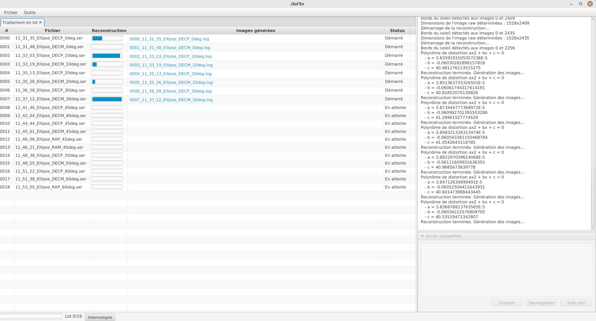
The file list for each SER file will include the log file for each video, as well as all generated images for that SER file.

In batch mode, we recommend that you pick a custom file name template which will output all images in a single directory: using the sequence number, this will make it easier to import into 3rd party software.

Reviewing batch processed images

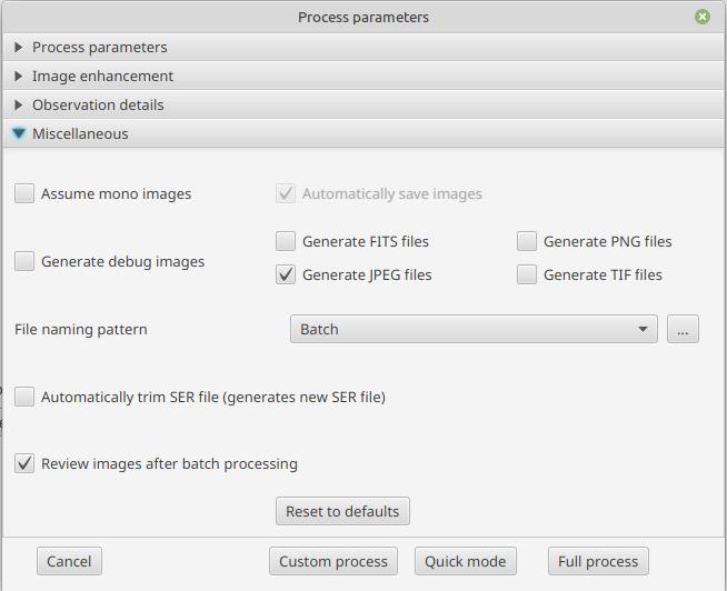
Once a batch has been processed, it is possible to review the generated images. This will make it possible, for example, to keep only images with a cloudless disk, or images without distortions.

In order to do so, in the processing options, in the "misc" tab, check the "Review images after batch processing" box:

Once processing is done, a new window will open, allowing you to review the processed images:

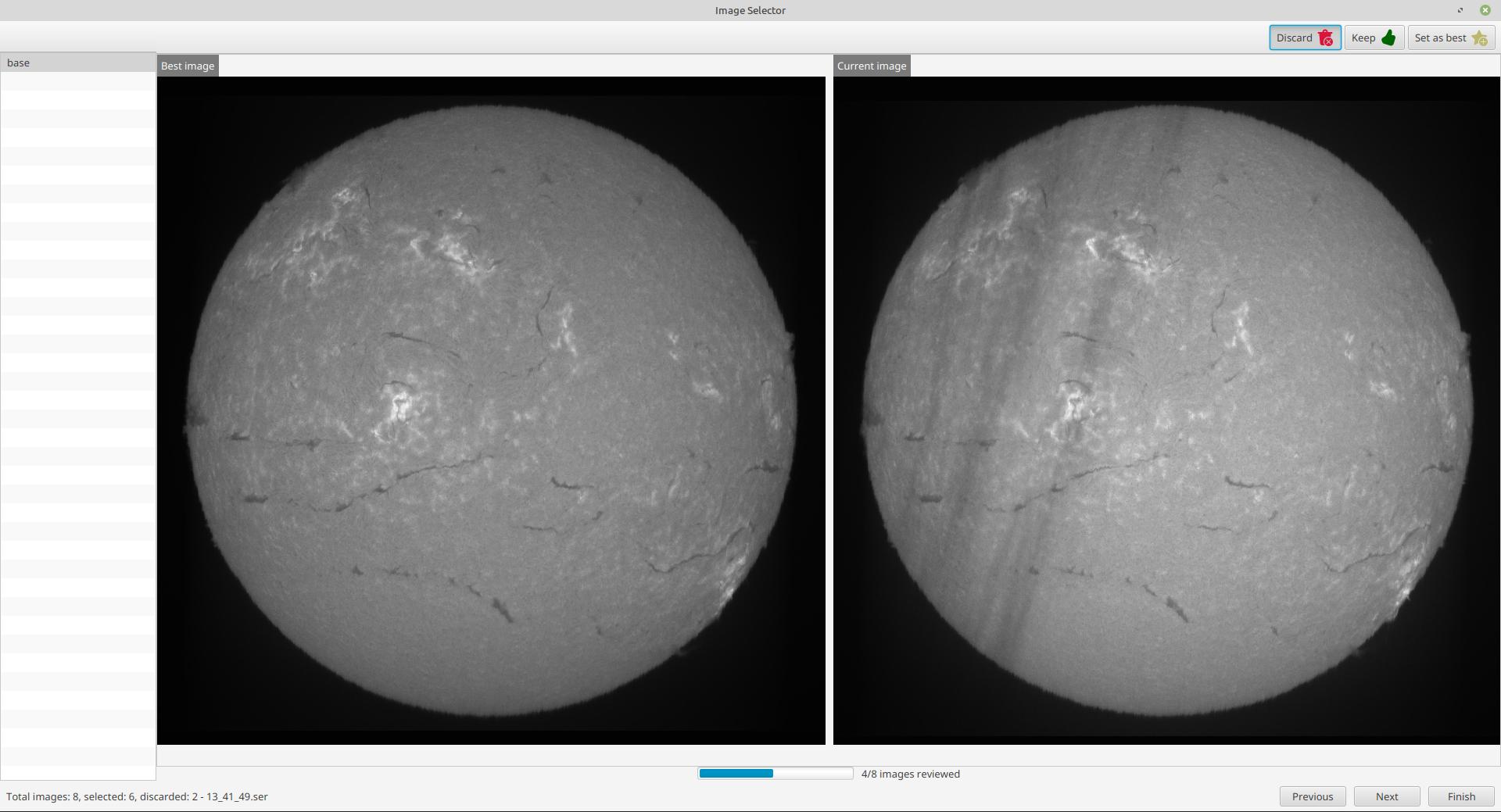
On the top right, you can choose to reject an image, keep it, or set it as the best image. The best image is then displayed on the left, and the current image on the right. You can then compare each image to the best image, and decide whether to keep it or not.

On the left, you have the list of images generated for each SER file. On the bottom right, you can move to the next or previous image, and finish the process.

Once you’re done, the following window will open:

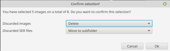
This lets you choose what you want to do with the rejected images: keep them, delete them, or move them to a sub-folder (by default, they will be moved). Similarly, you can choose what you want to do with the SER files which were used to generate these rejected images: keep them, delete them, or move them to a subfolder.

If you use a script in batch mode, the part of the script will only be executed for the images you have kept, which will allow, for example, stacking only the selected images.

Note that in the stack and stack_ref functions, you will then have the possibility to specify the reference selection method manual, which will then choose the best image you have selected.

ImageMath extensions available in batch mode

When you are in batch mode, an additional section is available in ImageMath scripts. This section allows making computations on the results of the processing of each individual image, in order to compose a final image for example (e.g stacking), or to create an animation of several images.

This section must appear at the end of a script and is introduced by the [[batch]] delimiter:

#
# Performs (simple) stacking of images in batch mode
#

[params]
# banding correction width and iterations
bandingWidth=25
bandingIterations=3
# autocrop factor
cropFactor=1.1
# contrast adjustment
clip=.8

[tmp]
corrected = fix_banding(img(0);bandingWidth;bandingIterations) (1)
contrast_fixed = clahe(corrected;clip)                         (2)

[outputs]
cropped = autocrop2(contrast_fixed;cropFactor;32)              (3)

# This is where we stack images, simply using a median
# and assuming all images will have the same output size
[[batch]]                                                      (4)
[outputs]
stacked=sharpen(median(cropped))                               (5)

1	For each SER file, we compute an intermediate corrected image (not stored on disk)
2	We perform contrast adjustment on the corrected images
3	Important for stacking: we crop the image to a square centered on the solar disk. The square has a width rounded to the closest multiple of 32 pixels. This is the output of each individual SER file processing.
4	We declare a `[[batch]]` section to describe the outputs of the batch itself
5	An image called `stacked` will be calculated by using the median value of each individual `cropped` image

It is important to understand that only the images which appear in the [outputs] section of the individual file processing are available for use in the [[batch]] section. Therefore, the cropped image of a single SER file becomes a list of images in the [[batch]] section. Some functions, like img are not available in the batch mode. If you need individual images to be available in the batch processing section, then you must assign them to a variable in the [outputs] section:

[outputs]
frame=img(0)       (1)

[[batch]]
[outputs]
video=anim(frame)  (2)

1	In order to make the `img(0)` image visible to the batch section, we must assign it to a variable that we call `frame`
2	An animation is created using each `frame`

Standalone scripts

An additional way to benefit from scripting is to reuse the results of previous sessions (typically, images produced in one or many previous sessions) without having to process a new video.

To do so, you must open the "Tools" menu and select "ImageMath editor". The interface which pops up is exactly the same as when you are processing a single video, or a batch of files. The main difference is how images are loaded. In this mode, you must use either the load or the load_many function to load images, instead of the img function.

If you use this mode, it is important to load images saved in previous sessions with the FITS format. These files include metadata such as the detected ellipse (solar disk), process parameters, etc. which will permit applying the same functions as you do in a standard processing session.

Measurements

Redshift Measurements

If you process an H-alpha image, JSol’Ex can automatically search within the image for regions where the redshift (red or blue shift) is particularly strong.

To do this, you must either select the "complete" mode during processing or check the "Redshift Measurements" box in the custom image selection.

The measurements will be valid only if the specified pixel size is correct and you are using a Sol’Ex (other spectroheliographs have different focal lengths).

During processing, an additional image will be generated with the regions outlined in red and the associated speed.

Additionally, if you select the debug images, the parts of the spectrum that allowed finding these regions will be displayed.

Finally, once the detection is complete, you can generate 2 new types of renderings by going to the "Redshift" tab:

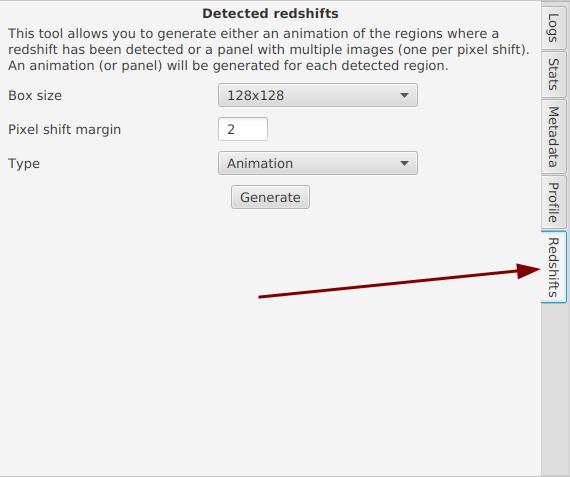
The size corresponds to the minimum size of the region to capture, in pixels. A small region will be centered around the detected filament, but it may be quite pixelated in some cases. The margin allows you to choose how many pixels to offset from what JSol’Ex detected. For example, JSol’Ex might find a maximum shift of 20 pixels, but you may wish to add 2 or 4 pixels of margin for an animation to clearly see the filament appear.

Finally, select the type of rendering:

Animation: generates a video where each frame is shifted by 0.25 pixels
Panel: generates a single image, a panel where each cell corresponds to a different pixel shift

Measurements thanks to the video analyzer

JSol’Ex provides a tool which will let you see what the detected spectral line is for a particular video. This tool chan be used, for example, to efficiently determine the pixel shift to apply when processing an Helium video.

To do this, open the "Video analyzer" in the "Tools" section. Select a video, the tool will compute the average image then show this window:

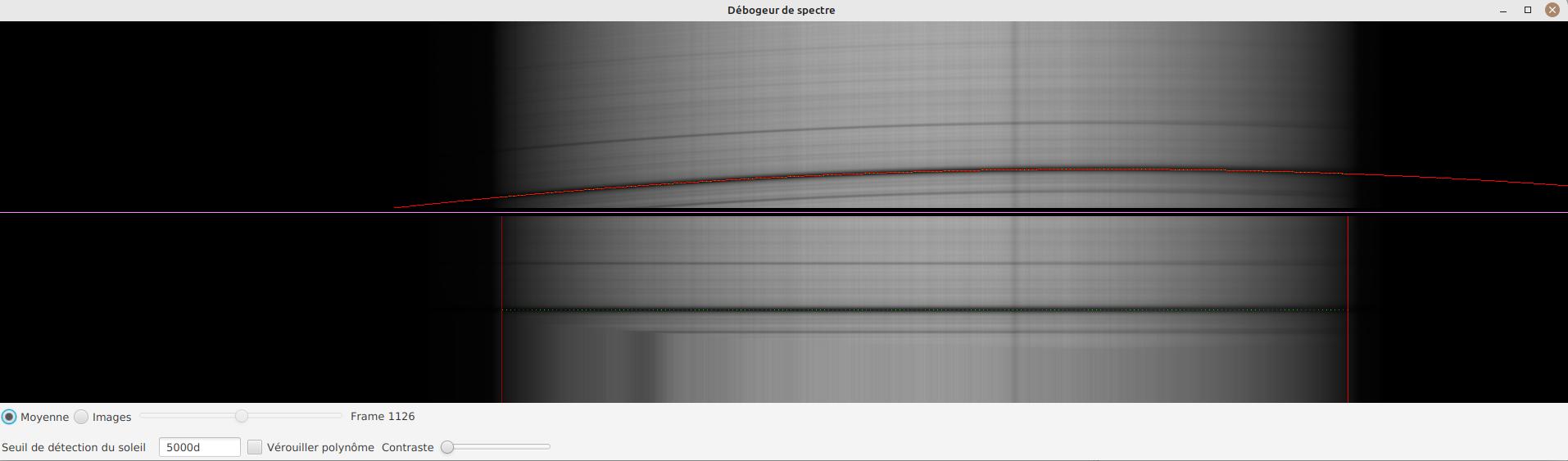
In the upper side you can see the reconstructed average image. The red line is the detected spectral ray, which is built by figuring out the darkest points of the lines. Below the violet line, you can see a geometry corrected version of the average image. If the line was properly detected, then the corrected image should show you perfectly horizontal lines.

In the lower part of the interface, you can adjust several parameters:

the "average"/"frames" radio buttons will let you choose between displaying the average image or the individual video frames
the sun detection threshold is a parameter you should avoid changing, since the software is not designed to override it in any case. It is provided for advanced debugging in case of bad recognition.
the "lock polynomial" checkbox will let us lock the current "red line" (a 2d order polynomial) as the one to use in all frames for display. We will use it in the helium ray spectral search below.
the "contrast" slider does what it says

Example of application to determine the helium ray pixel shift

We assume that we have a single SER file which window includes both the helium ray and another ray (e.g sodium) which is dark enough to be detected by JSol’Ex.

We can then proceed by steps:

first, lock the polynomial on the average image

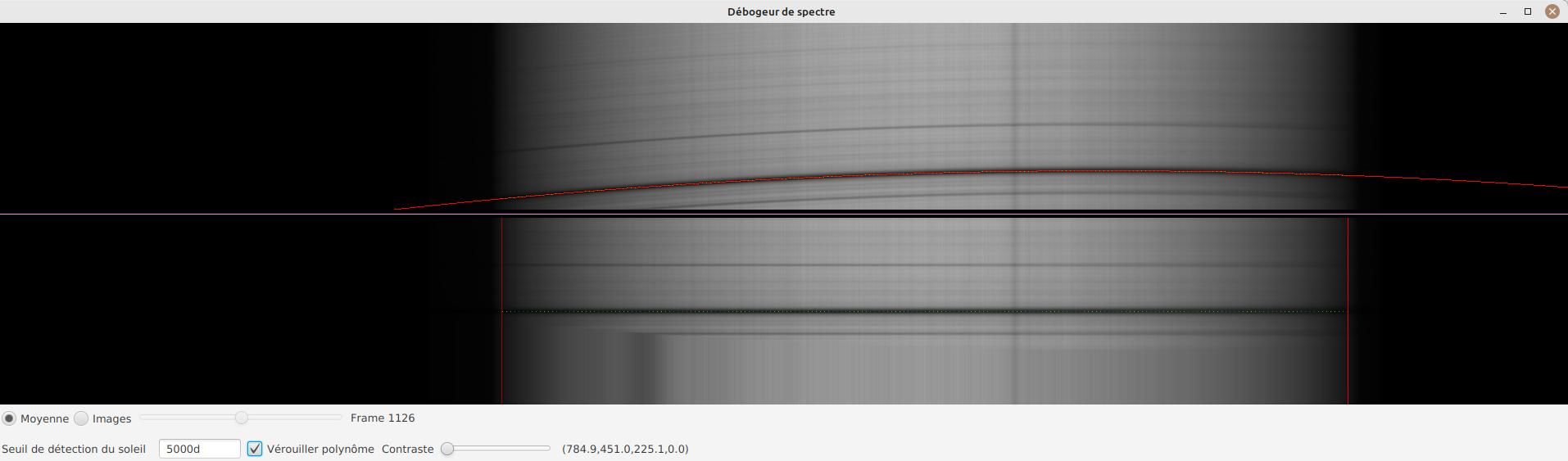
select the "Frames" mode

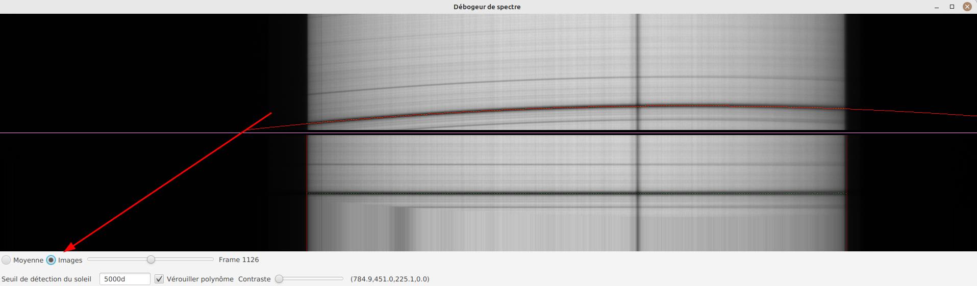
Adjust contrast to make the spectrum very bright

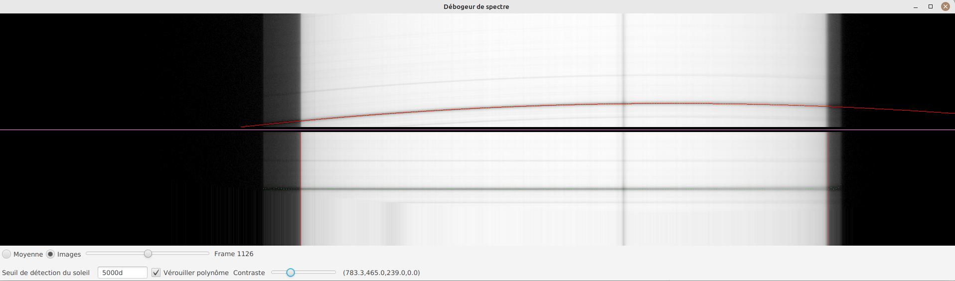
Select a frame which is close to the sun limb

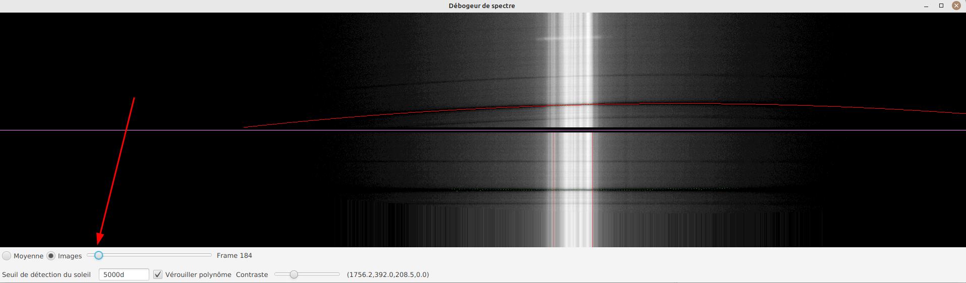
We can now perform measurements: when you are moving the mouse over the image, coordinates are displayed:

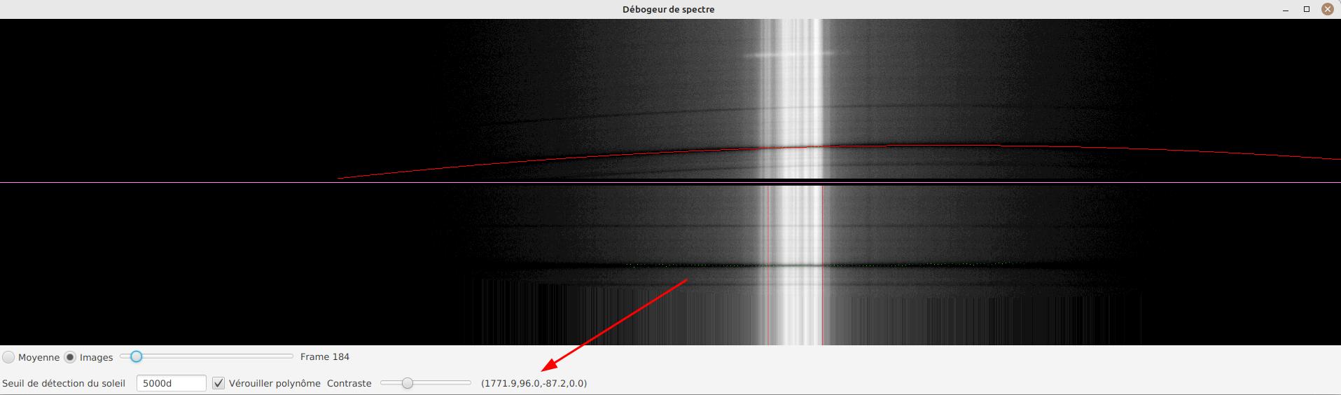
The first 2 numbers are the (x,y) coordinates of the point below the cursor. The 3rd one is the one we’re interested in: it’s the pixel shift between the cursor position and the detected spectral line (in red). The 4th number will let us increase our accuracy by computing an average value from samples.

To add a sample, find a point on the helium line then click on it while holding the CTRL key. You can add as many sample points as you wish.

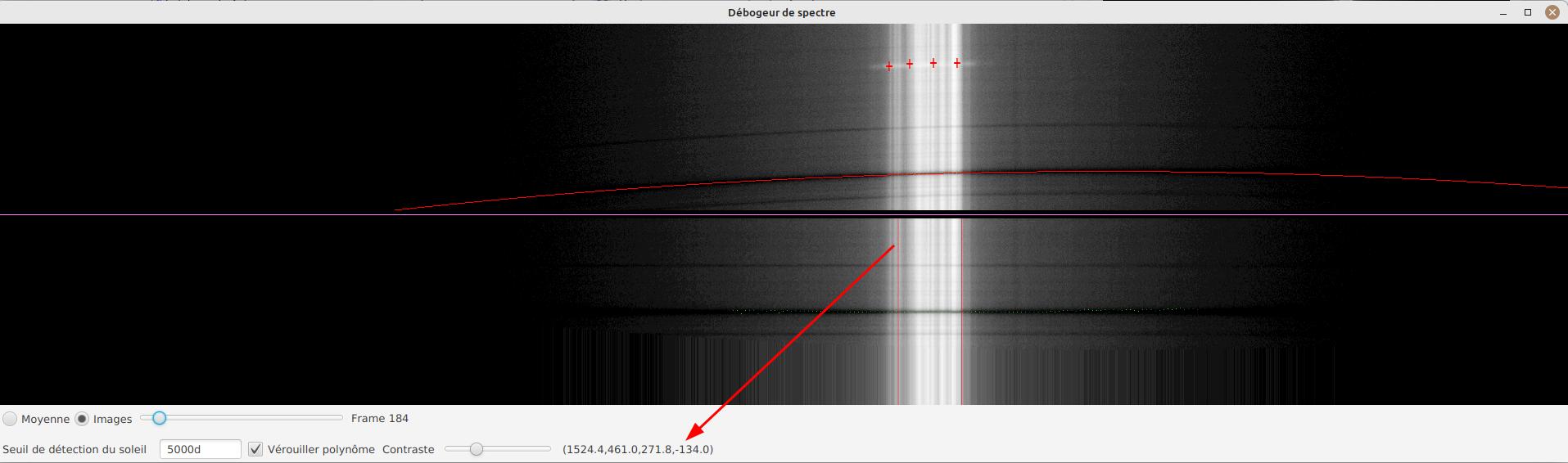
The 4th number is the average of distances and should be a good value to use in your ImageMath scripts. In this example we deduce that the pixel shift is -134.

Stacking and mosaic composition

JSol’Ex provides a tool to stack images and create mosaics. The 2 tools are very similar, but stacking is easier to use. Stacking consists of taking several images of a similar region of the sun and making a single image by aligning the details and averaging the pixels. Mosaics are similar, but they are used to create a single image from several images of different regions of the sun.

The 2 tools are available in the "Tools" menu, then "Stacking and mosaic composition".

The following window will show up:

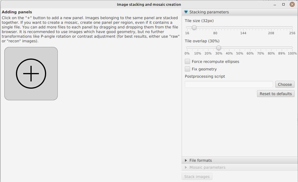
On the left, you can create image panels to stack. If you create a single panel, it will be a simple stacking. If you create several panels, each panel will be stacked, then a mosaic will be composed. A single panel can contain several images, which will be stacked together. To add a panel, click on the "+" button and select the images to stack. Alternatively you can drag and drop one or several images from your file explorer.

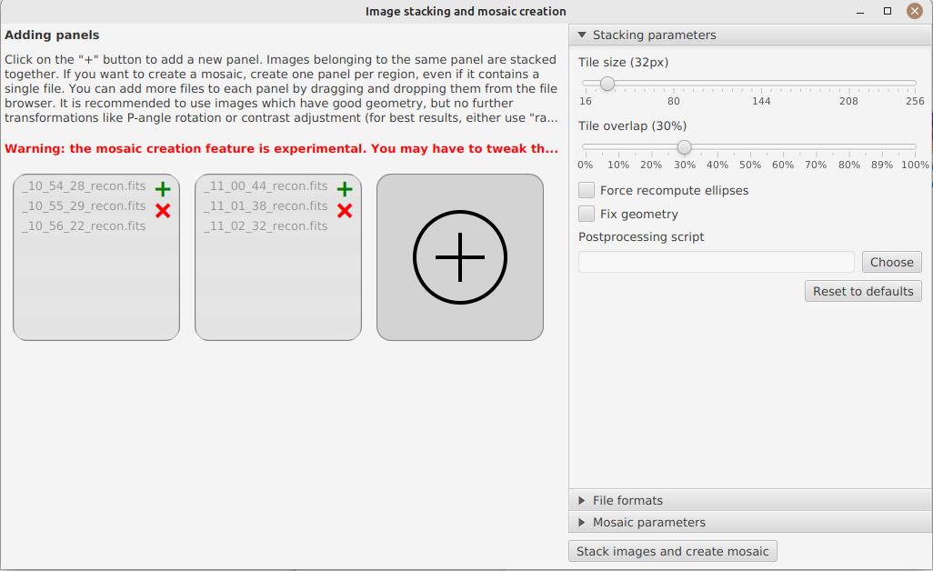
In the image above, we have created 2 panels. The first one contains 3 images which will be stacked to make the north panel, and the second one contains 2 images which will be stacked to make the south panel.

Stacking parameters are visible on the right. It is not recommended to change them, unless you know what you’re doing. The following options are available:

the tile size allows to cut the image in tiles for stacking. The smaller the tile size, the more precise the stacking will be, but the longer it will take and the less likely it will be able to compensate for large shifts between images.
the sampling factor determines where samples will be picked when computing the distorsion model. A sampling factor of 0.5 combined with a tile size of 32 means that a sample will be picked every 16 pixels.
Forcing the computation of ellipses can be useful if the images you import come from another software or if the ellipses were badly detected. In that case, we will recompute them before stacking.
Geometry correction should be applied on images which weren’t corrected before (e.g raw images).

The post-processing script is an ImageMath script that you can apply on each of the tiles after stacking.

In a post-processing script, the stacked image is available as image. For example, you can create a script which will apply a deconvolution using the formula rl_decon(image).

The other available options let you choose how files are saved. If you have created more than one panel, then the mosaic options become available.

For mosaic composition to work, it is recommended to use raw or recon images, not stretched ones. Indeed, stretched images are more difficult to align.

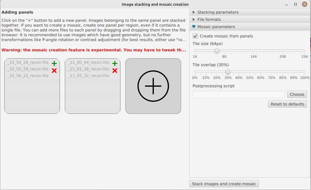
Should you only want to stack images without creating a mosaic, you can disable the "Create mosaic" option. In the other case, you can tweak some parameters, but it is strongly recommended not to change them unless the images you get after sticking are deformed or not reconstructed at all.

Again, you can apply a post-processing script to the mosaic.

Optimal exposure calculator

In the "tools" menu, you will find the optimal exposure calculator. This calculator will determine the optimal exposure time, in order to achieve a perfectly circular sun disk and avoid undersampling.

Enter the following parameters:

the camera pixel size (in microns) and the binning
the focal length of your instrument
the scan speed (a multiple of sideral speed, e.g 2, 4, 8, …)
the observation date

The software will then automatically compute the recommended framerate and the optimal exposure time in milliseconds.

Note that you can change the type of spectroheliograph used, which can change the calculation of the optimal exposure.

Spectrum Browser

The Spectrum browser is available in the "Tools" menu. It allows you to visualize the aspect of the spectrum as it would be seen in capture software such as SharpCap or FireCapture.

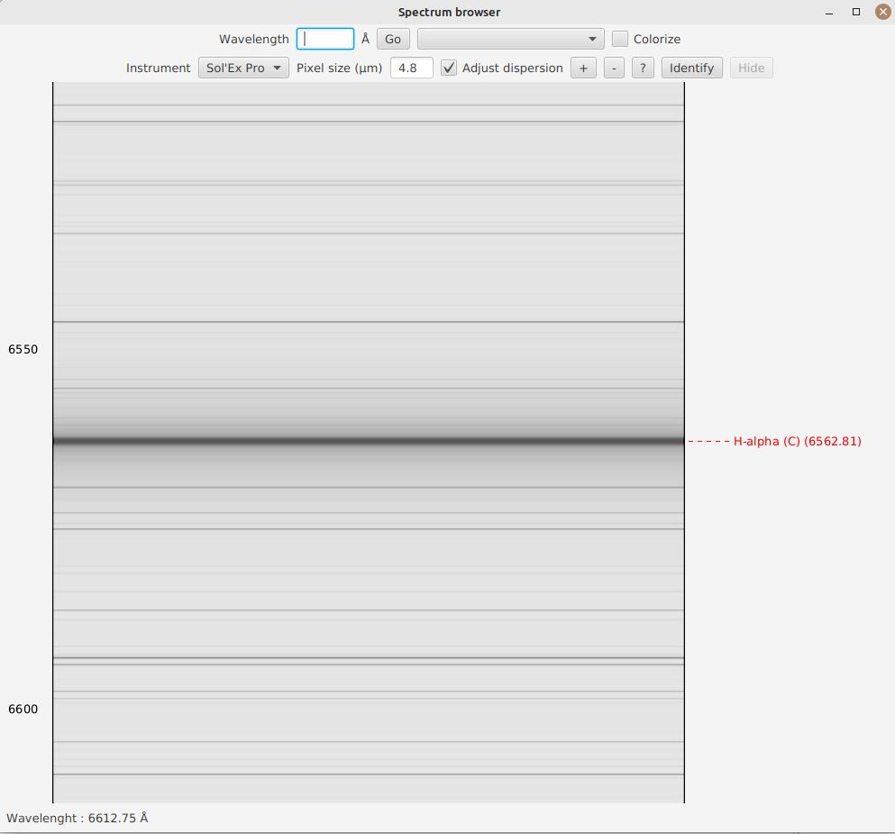
In the "Wavelength" box, you can enter a wavelength in Angstroms. By clicking "Go" or pressing enter, the spectrum will automatically center around this wavelength:

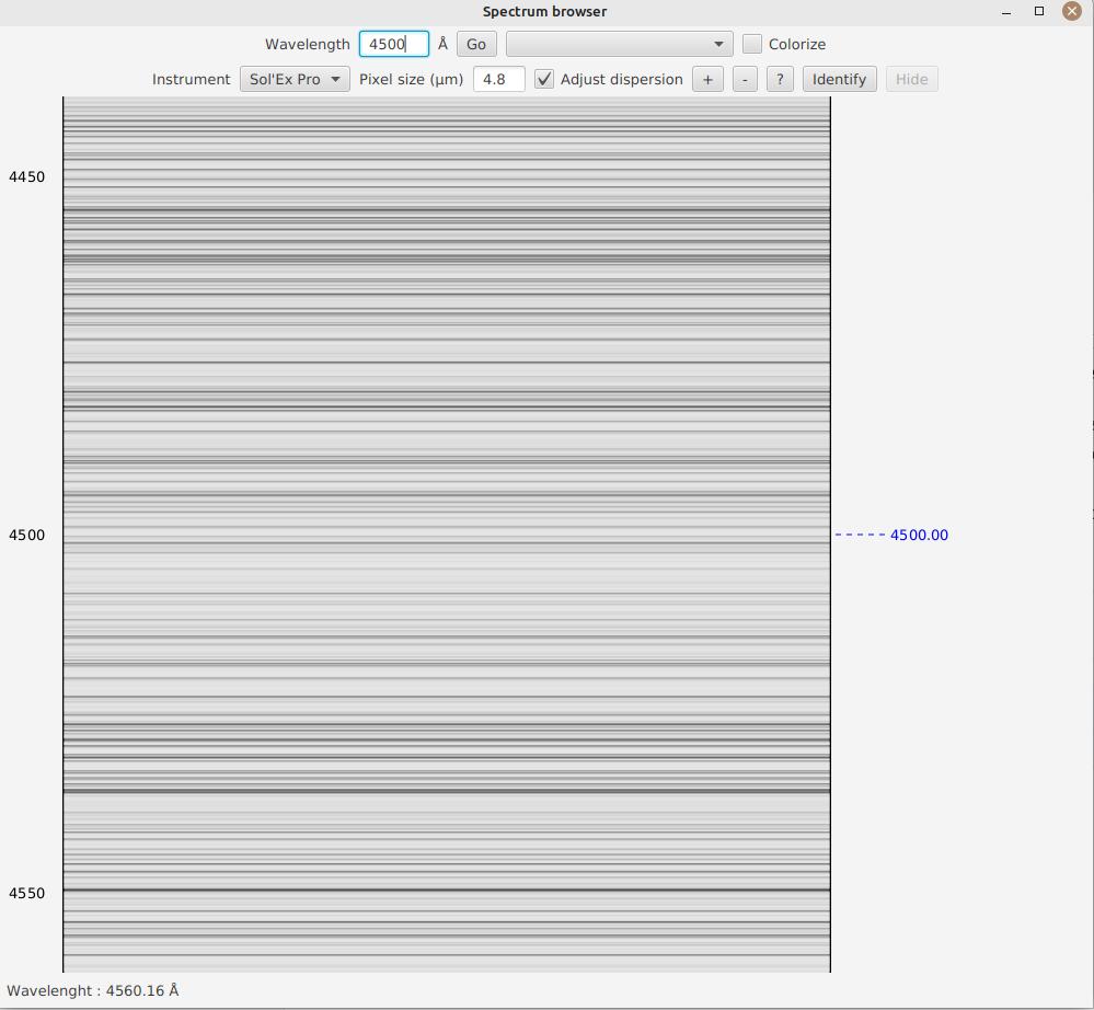
A blue dashed line is added, allowing you to clearly identify the line.

Alternatively, you can directly search for a notable spectral line by selecting it in the box next to the "Go" button.

When you click "Colorize", the spectrum is then colorized to give you an idea of where you are in the visible spectrum (however, we recommend staying in grayscale to precisely identify a line):

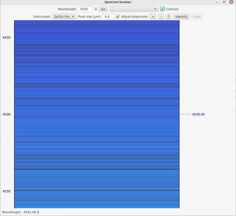
On the second line, you have the option to choose the spectroheliograph that is used (this will affect the calculated spectral dispersion), as well as to specify the pixel size (remember to multiply by the binning).

If you check the "Adjust Dispersion" box, the spectrum’s dimension is automatically adjusted to precisely match the calculated dispersion per pixel.

You can zoom either by clicking the "+" and "-" buttons, or more simply by pressing "CTRL" and scrolling your mouse wheel. If you zoom, the automatic adjustment is disabled (since it no longer corresponds to the exact dispersion per pixel).

Automatic Identification

Finally, JSol’Ex offers an experimental feature: you can click the "Identify" button to open a file selection window.

Then choose an image of the spectrum, as captured by your software. JSol’Ex will then try to find out which part of the spectrum it is in:

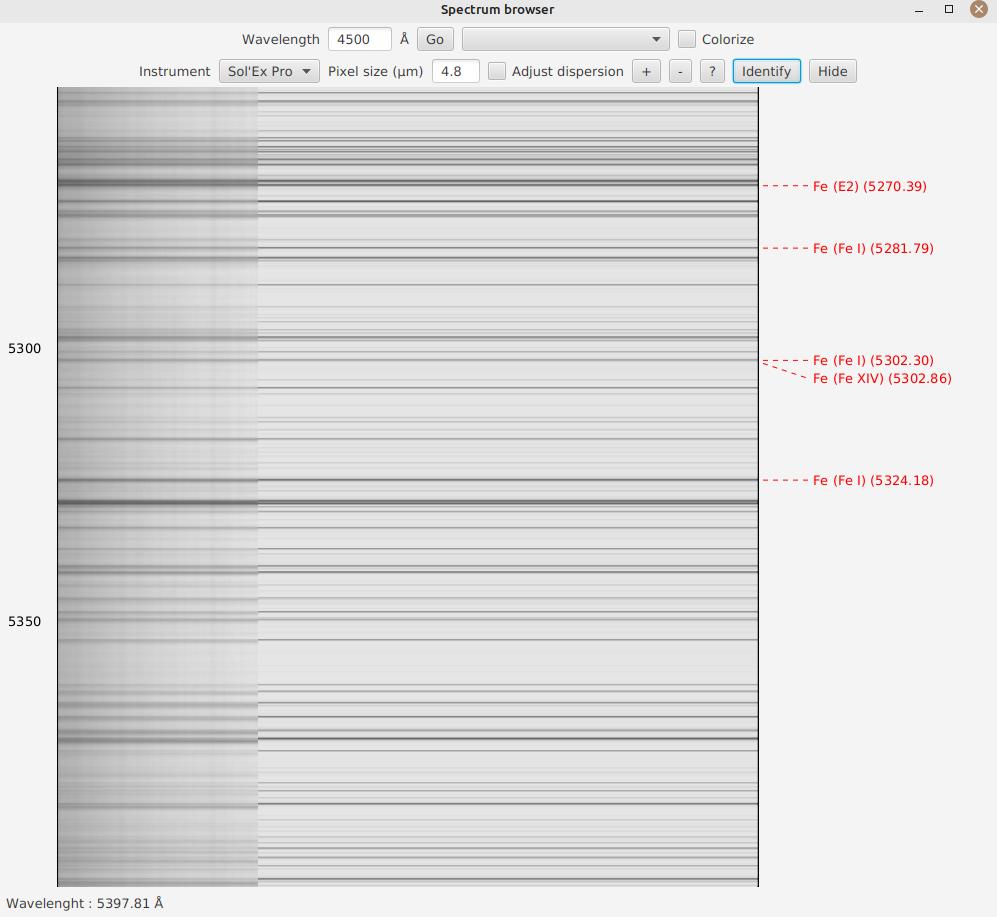
If the identification works, your image will be displayed in transparency, overlaid on the spectrum, on the left side of the image, allowing you to easily verify if the identification was successful.

You can hide the transparent image by clicking the "Hide" button.

Embedded Web Server

In the "Tools" menu, you will find the option to start an embedded web server. This server allows you to view images processed by the software from other computers, by connecting to this server.

This feature can be particularly useful during public presentations, with one computer using JSol’Ex for image acquisition and another computer on the same network for projection on a screen.

You can configure the port on which the server listens and have the option to start it automatically when the software starts.

The web UI gives access to images being processed as well as their history, in case you process several images successively.

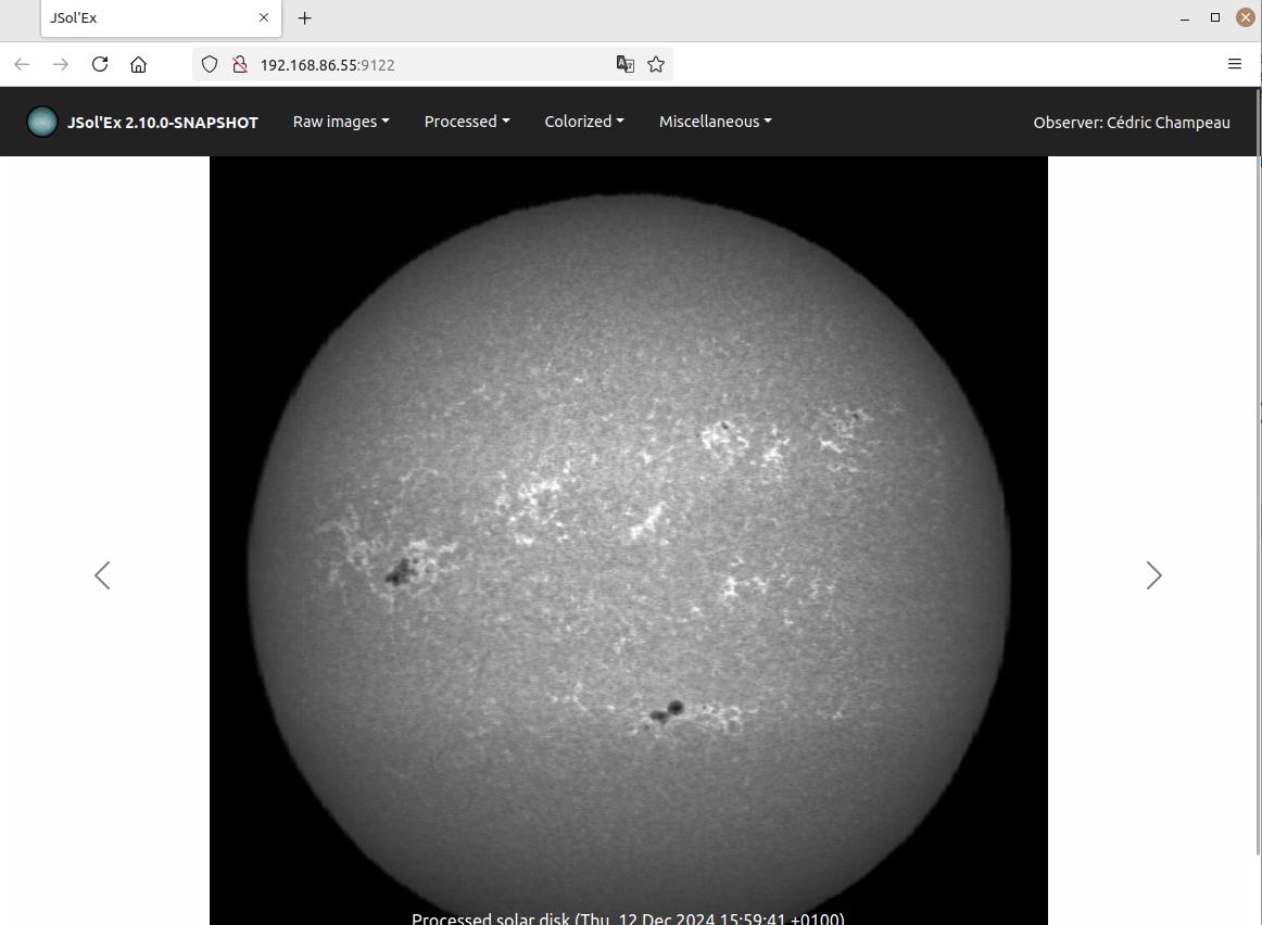
Acknowledgements

Christian Buil for designing Sol’Ex and leading the community with great expertise
Valérie Desnoux for her remarkable work on INTI
Jean-François Pittet for his bug reports, test videos, and geometric correction formulas
Sylvain Weiller for his intensive beta-testing, valuable feedback, and processing ideas
Ken M. Harrison for improved exposure time calculations