Stacking and mosaic creation with JSol’Ex 2.0
04 January 2024
Tags: astronomy astro4j solex java jsolex
A couple days ago I have released JSol’Ex 2.0. This software can be used as an alternative to INTI to process solar images acquired using Christian Buil’s Sol’Ex. This new version introduces 2 new features that I would like to describe in more details in this blog post: stacking and mosaic stitching.
Stacking
Stacking should be something familiar to anyone doing planetary imaging. One of the most popular sofware for doing stacking is AutoStakkert! which has recently seen a new major version. Stacking usually consists of taking a large number of images, selecting a few reference points and trying to align these images to reconstruct a single, stacked image which increases the signal-to-noise ratio. Each of the individual images are usually small and there are a large number of images (since the goal is to reduce the impact of turbulence, typically, videos are taken with a high frame rate, often higher than 100 frames per second). In addition, there are little to no changes between the details of a series (granted that you limit the capture to a few seconds, to avoid the rotation of the planet typically) so the images are really "only" disformed by turbulence. In the context of Sol’Ex image processing, the situation is a bit different: we have a few captures of large images: in practice, capturing an image takes time (it’s a scan of the sun which will consist of a video of several seconds just to build a single image) and the solar details can move quickly between captures. In practice, it means that you can reasonably stack 2 to 5 images, maybe more if the scans are quick enough and that there are not too many changes between scans.
The question for me was how to implement such an algorithm for JSol’Ex? Compared to planetary image stacking, we have a few advantages:
-
images have a great resolution: depending on the camera that you use and the binning mode, you can have images which range from several hundreds pixels large to a few thousands pixels
-
the images are well defined : in planetary observation, there are a few "high quality" images in a video of several thousand frames, but most images are either fully or partially disformed
-
there’s little movement between images: anyone who has stacked a planetary video can see that it’s frequent to see jumps of several pixels between 2 images, just because of turbulence
-
for each image, we already have determined the ellipse which makes the solar disk and should also have corrected the geometry, so that all solar disks are "perfect circles"
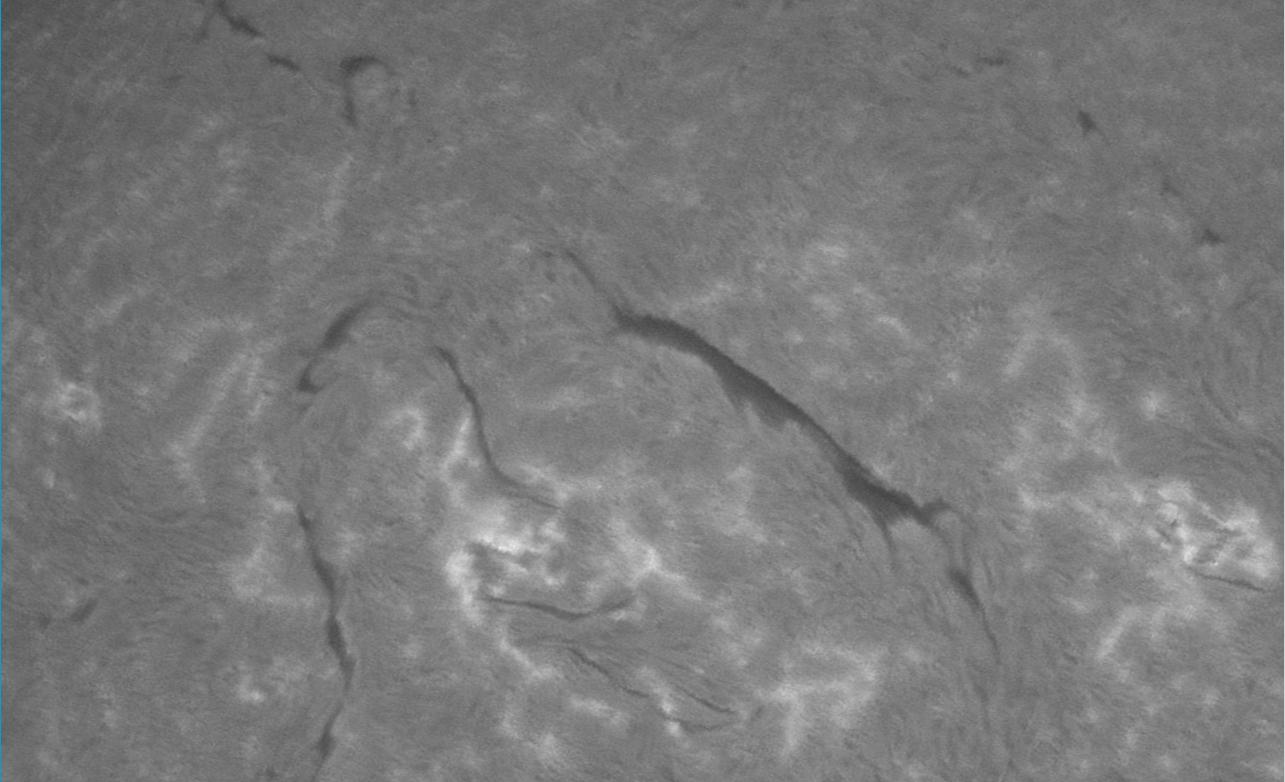
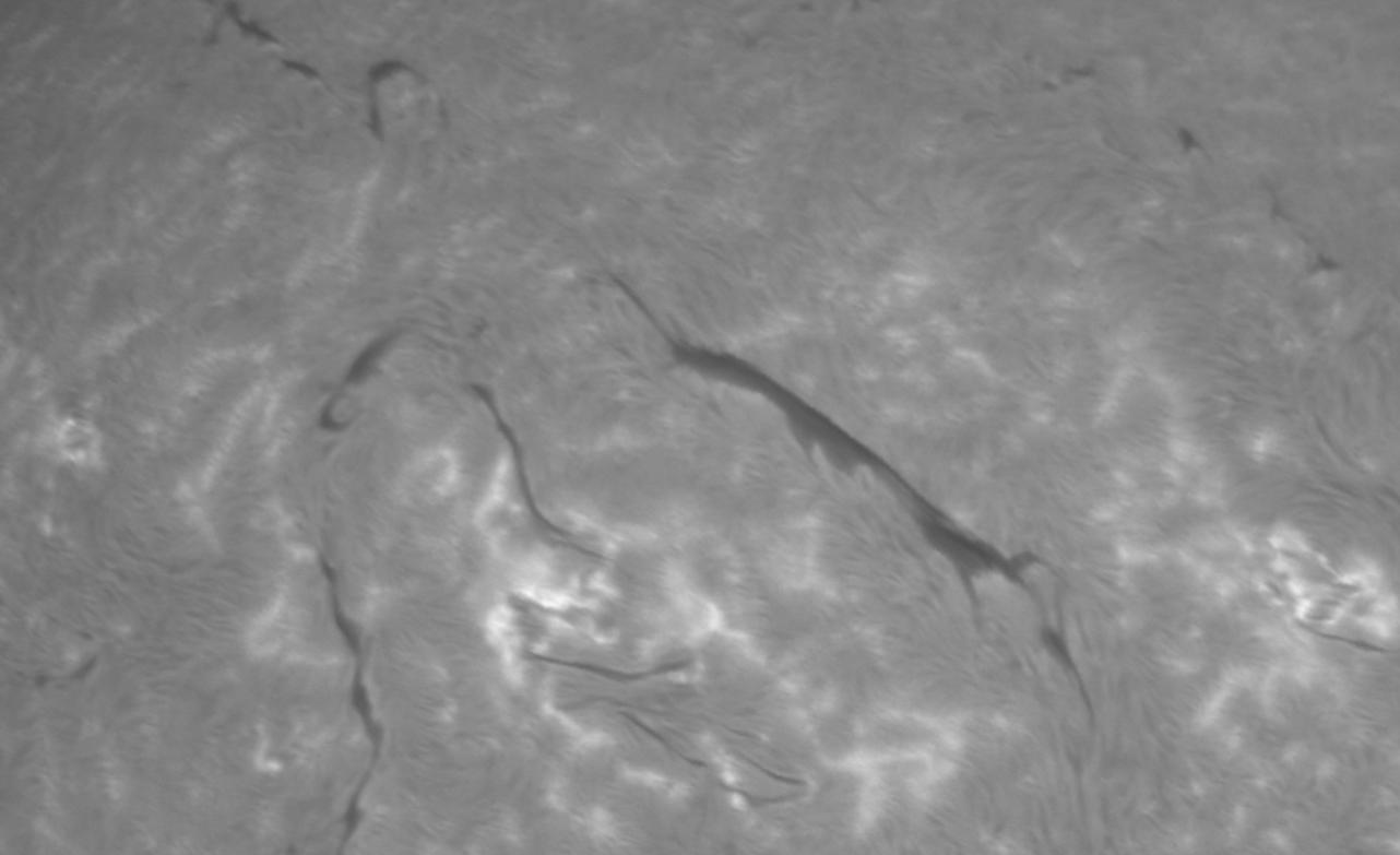
Therefore, a naive approach, which I tried without success a few months ago, is a geometric approach where we simply make all solar disks the same (by resizing), align them then create an average image. To illustrate this approach, let’s look at some images:
In this video we can see that there is quite some movement visible between each image. Each of them is already of quite good quality, but we can notice some noise and more importantly, a shear effect due to the fact that a scan takes several seconds and that we reconstruct line by line :
The average image is therefore quite blurry:
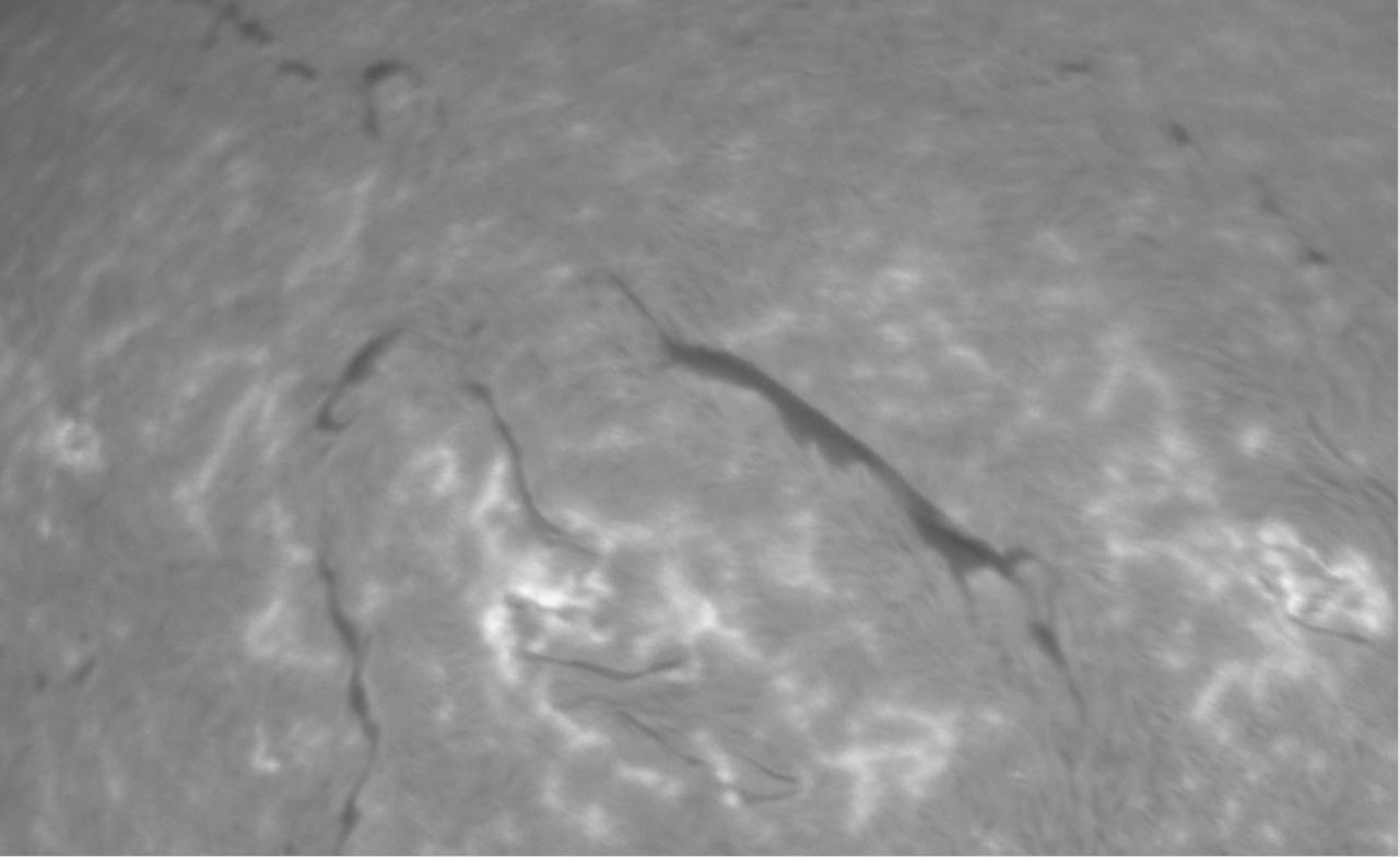
Therefore, using the average image is not a good option for stacking and that’s why I recommended to use AutoStakkert! instead, which gave better results.
In order to achieve better results, I opted for a simple yet effective algorithm:
-
first, estimate the sharpness of each image. This is done by computing the Laplacian of each image. The image with the best sharpness is selected as the reference image
-
divide each image into tiles (by default, a tile has a width of 32 pixels)
-
for each tile, try to align it with the reference image by computing an error between the reference tile and the image
-
the error is based on root mean squared error of the pixel intensities : the better the tiles are aligned, the closer to 0 the error will be
-
this is the most expensive operation, because it requires computing the error for various positions
-
we’re only looking for displacements with a maximum shift of 2/3 of the tile size (so, by default, 21 pixels maximum)
-
if the shift between 2 tiles is higher than this limit, we won’t be able to align the tiles properly
We could have stopped here and already reconstruct an image at this stage, but the result wouldn’t be great: the fact that we use tiles would be visible at the edges of the tiles, with square artifacts clearly visible. To reduce the artifacts, I opted for a "sliding window" algorith, where the next tile will overlap the previous one by a factor between 0 (no overlap) and 1 (100% overlap). This means that for each pixel, we will get a "stack" of pixel values computed from the alignment of several tiles. The final pixel value is then computed by taking the median value of the stack. Even so, some stacking vertical or horizontal artifacts can still be sometimes visible, so the last "trick" I used is to build the stacks by only taking pixels within a certain radius, instead of the whole square.
The resulting, stacked image is here:
We can see that:
-
noise from the original images is gone
-
shearing artifacts are significantly reduced
-
the resulting image is not as blurry as the average version
There were, however, some compromises I had to make, in order to avoid that the stacking process takes too long. In particular, the tile alignment process (in particular error computation) is very expensive, since for each tile, we have to compute 21*21 = 441 errors by default. With an overlap factor of 0.3, that’s, for an image of 1024 pixels large, more than 5 million errors to compute. Even computing them in parallel takes long, therefore I added local search optimization: basically, instead of searching in the whole space, I’m only looking for errors within a restricted radius (8 pixels). Then, we take the minimal error of this area and resume searching from that position: step by step we’re moving "closer" to a local optimum which will hopefully be the best possible error. While this doesn’t guarantee to find the best possible solution, it proved to provide very good results while significantly cutting down the computation times.
From several tests I made, the quality of the stacked image matches that of Autostakkert!.
Mosaic composition
The next feature I added in JSol’Ex 2, which is also the one which took me most time to implement, is mosaic composition. To some extent, this feature is similar to stacking, except that in stacking, we know that all images represent the same region of the solar disk and that they are roughly aligned. With mosaics, we have to work with different regions of the solar disk which overlap, and need to be stitched together in order to compose a larger image.
On December 7th, 2024, I had given a glimpse of that feature for the french astrophotograhers association AIP, but I wasn’t happy enough with the result so decided to delay the release. Even today, I’m not fully satisfied, but it gives reasonable results on several images I tried so decided it was good enough for public release and getting feedback about this feature.
Mosaic composition is not an easy task: there are several problems we have to solve:
-
first, we need to identify, in each image, the regions which "overlap"
-
then for each image, we need to be able to tell if the pixel value we read at a particular place is relevant for the whole composition or not
-
then we have to do the alignment
-
and finally avoid mosaicing artifacts, typically vertical or horizontal lines at the "edges"
In addition, mosaic composition is not immune to the problem that each image can have different illumination, or even that the regions which are overlapping have slightly (or even sometimes significantly) moved between the captures. Therefore, the idea is to "warp" images together in order to make them stitch smoothly.
Preparing panels for integration
Here are the main steps of the algorithm I have implemented:
-
resize images so that they all solar disks have the same radius (in pixels), and that all images are square
-
normalize the histograms of each panel so that all images have similar lightness
-
estimate the background level of each panel, in order to have a good estimate of when a pixel of an image is relevant or not and perform background neutralization
-
there can be more than 2 panels to integrate. My algorithm works by stitching them 2 by 2, which implies sorting the panels by putting the panels which overlap the most in front, then stitching the 2 most overlapping panels together. The result of the operation is then stitched together with the next panel, until we have integrated all of them.
The stitching part works quite differently than with typical stacking. In stacking, we have complete data for each image: we "only" have to align them. With mosaics, there are "missing" parts in the image that we need to fill in. To do this, we have to identify which part of a panel can be blended into the reconstructed image in order to complete it. This means that the alignment process is significanly more complicated than with typical stacking, since we will work on "missing" data. Part of the difficulty is precisely identifying if something is missing or not, that is to say if the signal of a pixel in one of the panels is relevant to the composition of the final image. This is done by comparing it with the estimated background level, but that’s not the only trick.
Despite the fact that our panels are supposedly aligned and that the circles representing the solar disks are supposed to be the same, in practice, depending on the quality of the capture and the ellipse regression success, the disks may be slightly off, with deformations. There can even be slight rotations between panels (because of flexions at capture time, or processing artifacts). As a consequence, a naive approach consisting of trying to minimize the error between 2 panels by moving them a few pixels in each direction like in stacking doesn’t work:
-
first of all, while you may properly align one edge of the solar disk, we can see that some regions will be misaligned. If these regions correspond to high contrast areas like filaments, it gives real bad results. If it happens at the edges of the sun, you can even see part of the disk being shifted a few pixels away from the other panel, which is clearly wrong.
-
second, estimating the error is not so simple, since we have incomplete disks. And in this case, the error has to be computed on large areas, which means that the operation is very expensive.
-
third, because we have to decide whether to pick a pixel from one panel or the other, this has the tendency to create very strong artifacts (vertical or horizontal lines) at the stitching edges
The stitching algorithm
Giving all the issues I described above, I chose to implement an algorithm which would work similarly to stacking, by "warping" a panel into another. This process is iterative, and the idea is to take a "reference" panel, which is the one which has the most "relevant" pixels, and align tiles from the 2d panel into this reference panel.
To do this, we compute a grid of "reference points" which are in the "overlapping" area. These points belong to the reference image, and one difficulty is to filter out points which belong to "incomplete" tiles. Once we have these points, for each of them, we compute an alignment between the reference tile and the tile of the panel we’re trying to integrate. This gives us, roughly, a "model" of how tiles are displaced in the overlapping area. The larger the overlapping area is, the better the model will be, but experience shows that distorsion on one edge of the solar disk can be significanly different at the other edge.
The next step consists of trying to align tiles of the panel we integrate to the reference panel using this model. This is where the iteration process happens. In a nutshell, we have an area where the solar disk is "truncated". Even if we split the image in tiles like with stacking, we cannot really tell whether a tile is "complete" or not, because it depends both on the pixel intensities of the reference panel and the second panel, and the background level. In particular, calcium images may have dark areas within the solar disk which are sometimes as dark as the background.
If you are struggling to understand how difficult it can be to determine if part of the image we consider is relevant or not, let’s illustrate with this image:
Can you see what’s wrong in this image? Let’s increase constrast to make it clearly visible:
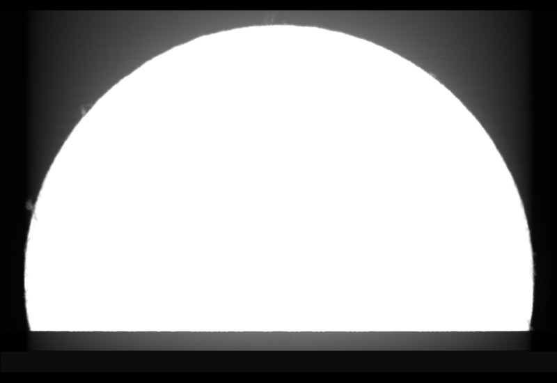
Now it should be pretty obvious that below the south edge of the truncated disk, we have an area which has pixels which are above the value of the background, but do not constitute actual signal! This problem took me quite some time to solve, and it’s only recently that I figured out a solution: before mosaicing, I am performing a background neutralization step, by modeling the background and substracting it from the image. While this doesn’t fully solve the problem, it makes it much less relevant for composition.
In addition, we have to compose the image using tiles which are incomplete, and we don’t know the orientation of the panels: they can be assembled north/south, or west/east, and nothing tells us. Potentially, it can even be a combination of these for a large number of panels.
Therefore, the algorithm works by creating a "mask" of the image being reconstructed. This mask tells us "for this particular pixel, I have reconstructed a value, or the value of the reference image is good enough and we won’t touch it". Then, for each tile, we consider tiles for which the mask is incomplete.
In order to determine how to align the truncated disk with data from the other image, we compute an estimate of the distortion of the tile based on the displacements models we have determined earlier. Basically, for a new "tile" to be integrated, we will consider the sample "reference points" which are within a reasonable distance of the tile. For this set of reference points, we know that they are "close enough" to compute an average model of the distorsion, that I call the "local distorsion": we can estimate, based on the distance of each reference point, how much they contribute to the final distorsion model for that particular point.
The key is really to consider enough samples to have a good distorsion model, but not too many because then the "locality" of alignment would become too problematic and we’d face misalignments. Because there are not so many samples for each "incomplete" tile, we are in fact going to reconstruct, naturally, the image from the edges where there’s missing data: when there are no samples, it basically means we cannot compute a model, so we don’t know how to align tiles. If we have enough samples, then we can compute a reliable model of the distorsion, and then we can reconstruct the missing part of each tile, by properly aligning the tiles together. If the number of samples is not sufficient to consider a good model, then we assume that no distorsion happens, which is often the case for "background" tiles.
Most of the difficulty in this algorithm is properly identifying "when" we can stitch tiles together, that is to say when we can tell that the alignment between tiles makes sense and that the alignment is correct. Often, I got good results for one kind of images (e.g, h-alpha images) but horrible results with others (e.g calcium) or the other way around. I cannot really say I took a very scientific approach to this problem, but more an empirical approach, tweaking parameters of my algorithm until it gave good enough results in all cases.
I mentioned that the algorithm is iterative, but didn’t explain why yet: when we compute the tile alignments, we only do so because we have enough local samples for alignment. We do this for all tiles that match this criteria, but we won’t, for example, be able to align a tile which is in the top of the image, if the bottom hasn’t been reconstructed. Therefore, the iteration happens when we have reconstructed all the tiles we could in one step: then we recompute new reference points, and complete the image, not forgetting, of course, to update our mask to tell that some pixels were completed.
Overall the algorithm is fairly fast, and can be stopped once we have completed all tiles, or after a number of fixed iterations in case of difficulties (often due to the background itself).
One last step
The algorithm we’ve described provides us with a way to "roughly" reconstruct an image, but it doesn’t work like what you’d intuititvely think of mosaic composition, by "moving" 2 panels until they properly align and blend them toghether. Instead, it will reconstruct an image by assembling tiles together, from what is already reconstructed: it is more fine grained, which will fix a number of the issues we’ve faced before: local distorsions, or images which are not properly aligned because the details at the surface at the sun have moved between the moment the first panel was captured and the second one did.
If we stopped there, we would see an image which looks like this:
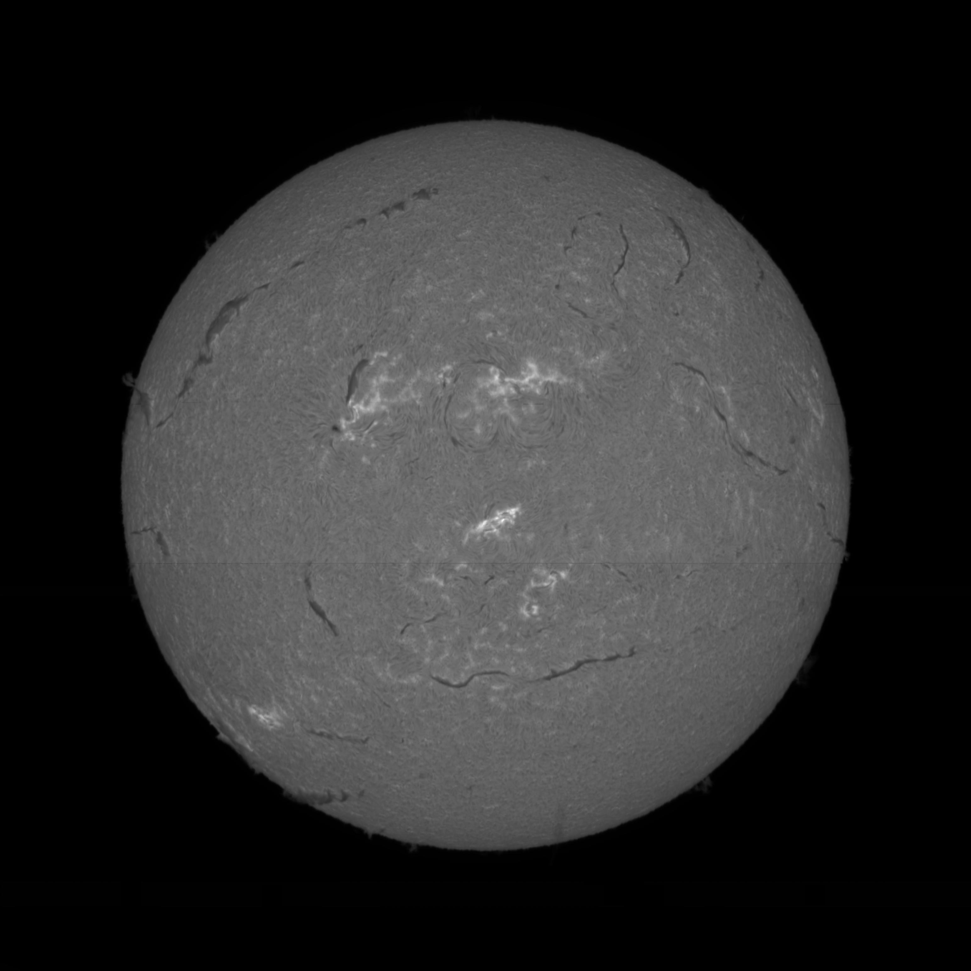
We can see a clear horizontal line, which is due to the fact that we’re reconstructing using tiles, and that depending on the alignment of tiles with the "missing" areas, we can have strong or weak artifacts at the borders. Errors are even more visible in this image in calcium K line:
This time it’s very problematic and we are facing several of the issues we attempted to avoid: details have significantly moved between the north and south panel were captured, which leads to "shadowing" artifacts, and there are also tiling artifacts visible.
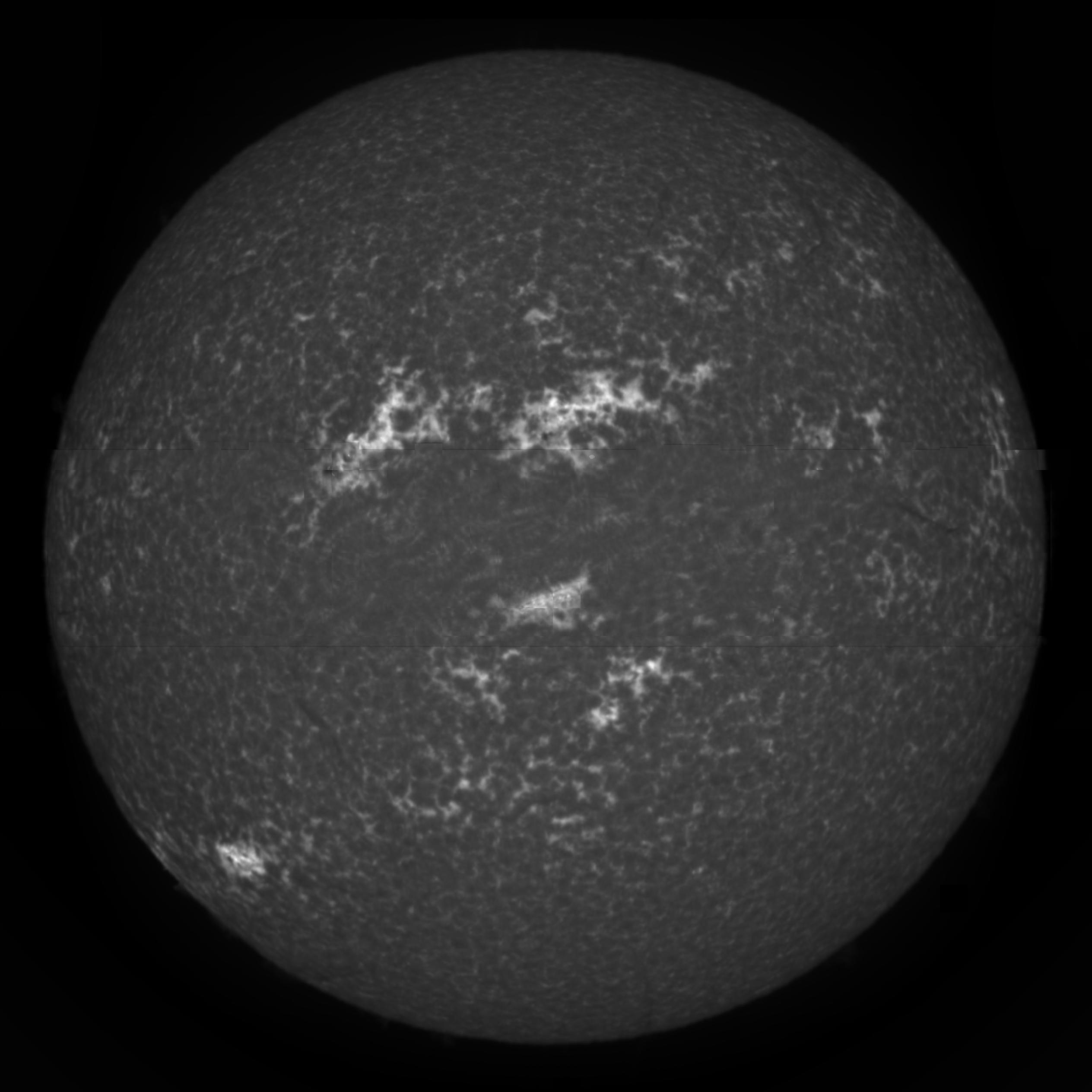
However, the image we get is good enough to perform one last step: use it as a reference image in the stacking algorithm we described in the first section of this blog post. The reason stacking works well is because we know we have complete images that we can align. Here, we have roughly reconstructed an image that we can use as a "complete reference". The idea is therefore to take each tile of each panel and "blend" it using the reconstructed reference. Of course, there is one big difference between the stacking in the first section and the stacking we have to do now. We’re not really going to use the reconstructed image, except for aligning tiles together and computing a "weight" for each tile, which depends on the relative luminosity between the reference image tile we’re considering and the corresponding panel tile.
This gives us a pretty good result:

The images we got there are not perfect, which is why I’m not fully satisfied yet, but they are however already quite good, given that it’s all done in a few seconds, using the same software that you’d use to reconstruct Sol’Ex images! In other words, the goal of these features is not to get the same level of quality that you’d get by using your favorite post-processing or mosaic composition software, but good enough to get you a reasonable result in a reasonable amount of time.
For example, on my machine, it takes less than one minute to:
-
stack images of the north and south panels (~10 images to stack)
-
stitch them together in a mosaic
It would have taken several minutes, or even more, using external software, especially for the mosaic part.
Conclusion
In this blog post, I have described how I got to implement 2 algorithms, the stacking algorithm and the mosaic composition one, in JSol’Ex. None of the algorithms were based on any research paper: they were really designed in an "adhoc" way, as my intuition of how things could work. It proved to be quite difficult, and it is very likely that better algorithms are described in the wild: I will consider them for future versions.
Nevertheless, I’m quite happy with the outcome, since, remember, I have started this program as an experiment and for learning purposes only. Now I sincerely hope that it will help you get amazing solar images!
