Jagged Edges Correction with JSol’Ex 3.1

Spectroheliographs like the Sol’Ex or the Sunscan are not using a traditional imaging system like, for example, in planetary imaging, where you can capture dozens to hundreds of frames per second and do the so called "lucky imaging" to get the best frames and stack them together to get a high resolution image.

In the case of a spectroheliograph, the image is built by scanning the solar disk in a series of "slices" of the sun: it takes several seconds and sometimes minutes (~3 minutes when you let the sun pass "naturally" through the slit) to get a full image of the sun.

In practice, this means that between each frame, each "slice" of the sun, the atmosphere will have slightly moved, causing some misalignment between the frames. This is also particularly visible when there is some wind, which can cause the telescope to shake a bit, and the image to be misaligned. Lastly, you may even have a mount which is not perfectly balanced, or which has some resonance at certain scan speeds.

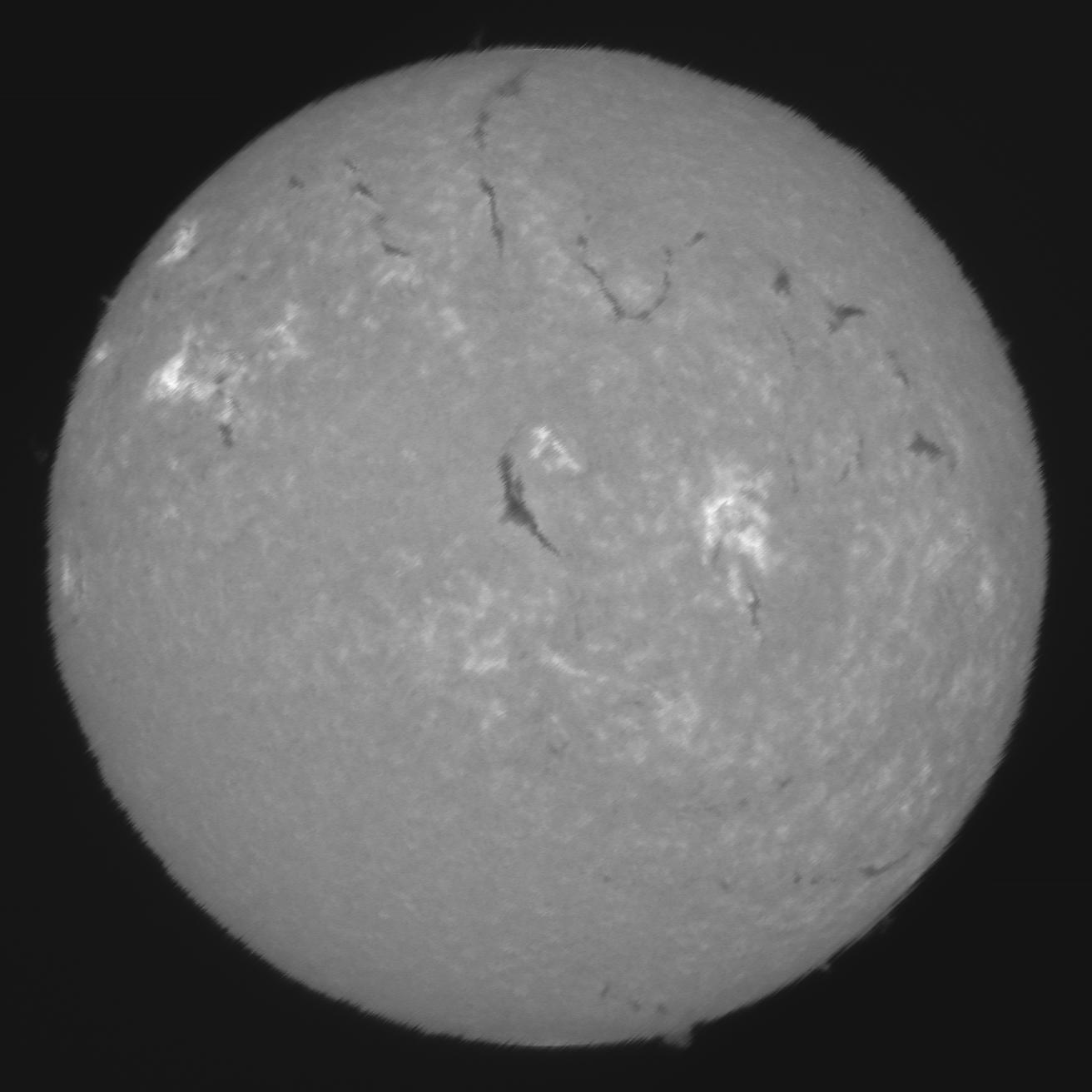
As an illustration, let’s take this image captured using a Sunscan (courtesy of Oscar Canales):

This image shows 3 problems:

These issues are typical of spectroheliographs, and are the main limiting factor when it comes to achieving high resolution images. Therefore, excellent seeing conditions are a must to get high quality images. Even if you do stacking, the fact that the reference image will show spikes is often a problem.

Starting with release 3.1.0, JSol’Ex ships with an experimental feature to correct jagged edges. It is not perfect yet, but good enough for you to provide feedback and even improve the quality of your images.

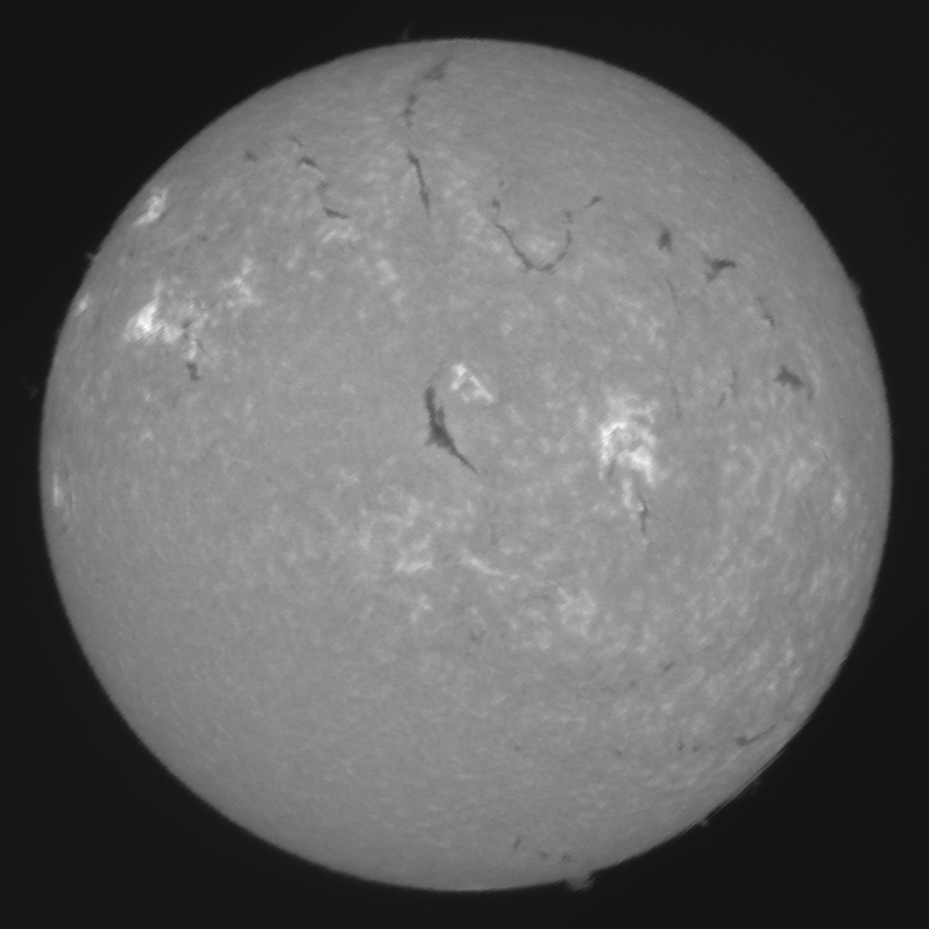
For example, here’s the same image, but with jagged edges correction applied:

And so that it’s even easier to see the difference, here’s a blinking animation of the two images:

The jagged edges are now mostly gone, the features in the sun are better aligned, and the image is much more pleasant to look at. There is still some jagging visible, the correction will never be perfect, but it is a good start.

In particular, you should be careful when applying the correction, because it could cause some artifacts in the image, in particular on prominences. As usual, with great powers comes great responsibilities!

To illustrate how the correction works, let’s imagine a perfect scan: a scan speed giving us a perfectly circular disk, no turbulence, no wind, etc.

In this case, what we would see during the scan is a spectrum which width slowly increases, reaches a maximum, and then decreases. The pace at which the width increases and decreases is determined by the scan speed and is predictable. In particular, the left and right borders of the spectrum will follow a circular curve.

Now, let’s get back to a "real world" scan. In that case, the left and right edges will slightly deviate from the circular curve. They will also follow the path of an ellipse: in fact, this ellipse is already required in order to perform geometric correction.

The idea is therefore quite simple in theory: we need to detect the left and right edges of the spectrum, then compare them to the ideal ellipse that we have computed. Pixels which deviate from this curve give us an information about the jagged edges. We can then compute a distortion map, which will be used to correct the image.

In practice, we also need to apply some filtering of samples: in practice, while the detection of edges is robust enough to provide us with a good geometric correction, it is not perfect. It can also be skewed by the presence of proms for example. Therefore, we are performing a sigma clipping on the detected edges, in order to remove outliers, that is to say pixels which deviate too much from the average deviation.

This is also why the correction will not work properly if the image is not focused correctly: you would combine two problems in one, and the correction would not be able to detect the edges properly.

In addition, in the image above you can see that the bottom most prominence is slightly distorted, which is caused by the fact that it’s far away from the 2 points which were used to compute the distortion. It may be possible to reduce such artifacts by using a smaller sigma factor (at the risk of undercorrecting edges).

In this blog post, I have described the new jagged edges correction feature in JSol’Ex 3.1. This solves one of the most common issues users are having with spectroheliographs, and I hope it will help you get better images. However, as usual, it’s a work in progress, so do not hesitate to provide feedback!