Cédric Champeau's blog: Ellerman Bombs Detection with JSol’Ex 3.2

About Ellerman Bombs

Ellerman bombs were first described by Ferdinand Ellerman back in 1917. Ellerman’s article was named -Solar Hydrogen "Bombs"- and it’s only later that these were commonly referred to as "Ellerman bombs".

I came upon this term while reading an article from Sylvain or André Rondi quite early in my solar imaging journey, and I was since then obsessed by these phenomena.

Ellerman Bombs are small, transient, and explosive events that occur in the solar atmosphere, particularly in the vicinity of sunspots. These are very short lived compared to other solar features: from several dozens of seconds to a few minutes. The most common explanation is magnetic reconnection, which occurs when two magnetic regions opposite polarity come into contact and reconnect, releasing energy in the form of heat and light. This is for example described in this article from González, Danilovic and Kneer.

Amateur observations of Ellerman bombs are quite rare, but Rondi described such observations using a spectroheliograph back in 2005. They are rare because they are mostly invisible where the amateur observations are made (the center of the H-alpha line), and are too small to notice. However, these are visible in the wings of the H-alpha line: this is where a spectroheliograph comes in handy, since the cropping window that is used to capture an image contains more than just the H-alpha line.

I had a long standing issue to do something about it in JSol’Ex, and I finally got around to it: all it took was getting some test data to entertain the ideas.

Observation of an Ellerman Bomb

I am doing many observations of the sun: I started in 2023 with a Sol’Ex, then I recently got an SHG 700, so I have accumulated quite a bit of data, which is completed by scans which are shared with me by other users of JSol’Ex.

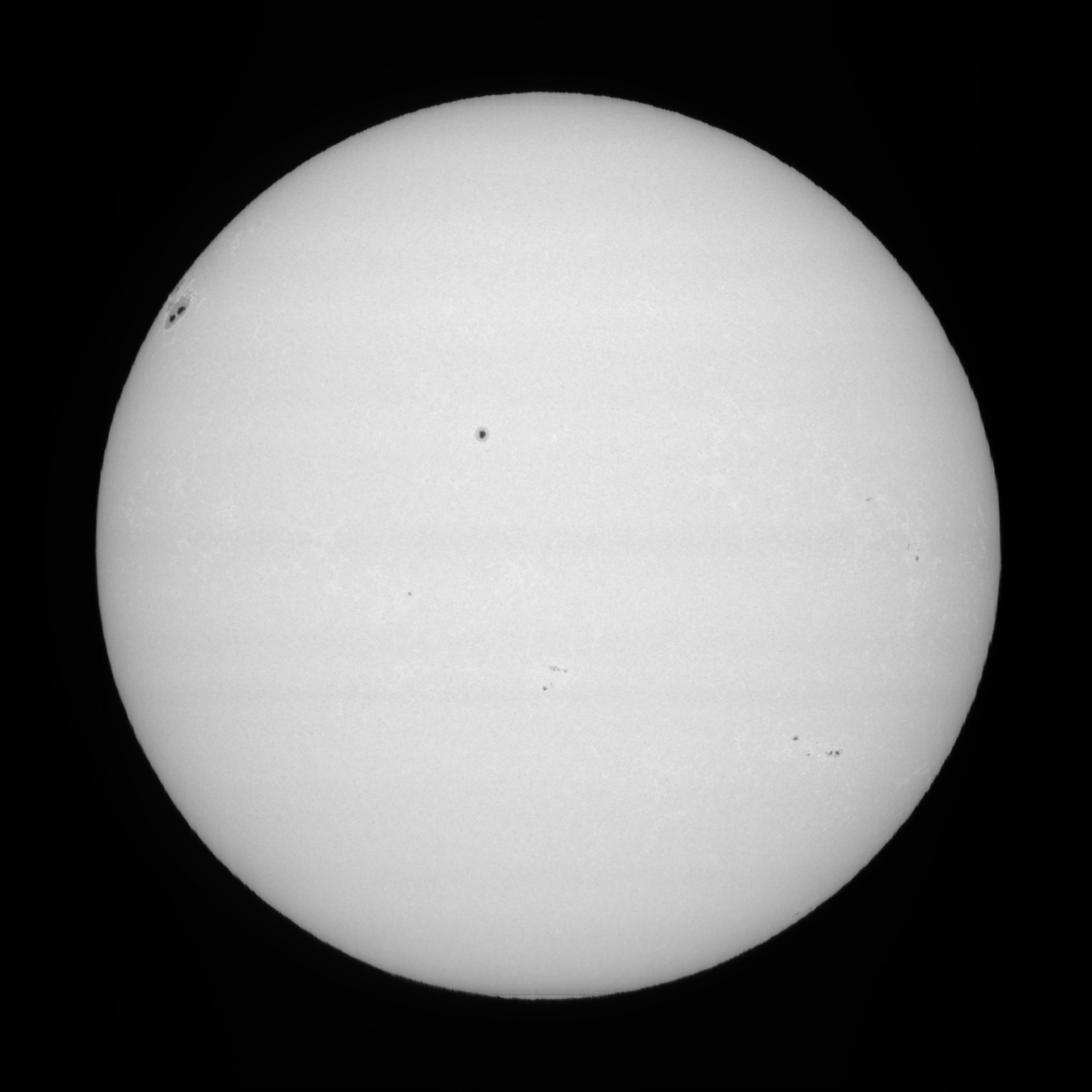
I have been looking for Ellerman bombs in my data, but I never found any yet. This changed a couple weeks ago: I was doing some routine work on JSol’Ex and using a capture I had done in April, 29, 2025 at 08:32 UTC, when I noticed, by accident, a bright spot in the continuum image:

It may not be obvious at first, which is precisely why these are hard to spot, so here’s a hint:

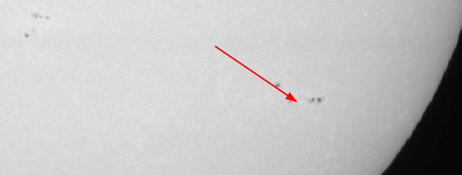
JSol’Ex offers the ability to easily generate animations of the data captured at different wavelengths, so I generated a quick animation, which shows the same image at ±2.5Å from the center of the H-alpha line:

We can see the typical behavior of an Ellerman bomb: it is bright in the wings of the H-alpha line, but it vanishes when we are at the center of the line. The fine spectral dispersion of the spectroheliograph makes it possible to highlight this phenomenon very precisely.

The corresponding frame of the SER file shows the aspect of the Ellerman bomb in the spectrum:

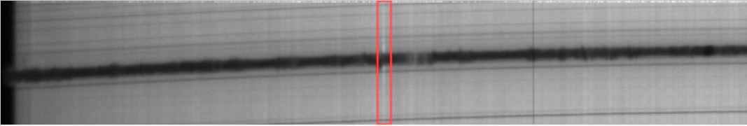
The shape that you can see is often referred to as the "moustache". At this stage I was pretty sure I had observed my first Ellerman bomb, and that I could implement an algorithm to detect it.

JSol’Ex 3.2 auto-detection

JSol’Ex 3.2 ships with a new feature to automatically detect Ellerman bombs in the data. Currently, it is limited to H-alpha, but it should be possible to detect these in CaII as well.

The algorithm I implemented uses statistical analysis of the spectrum to match the characteristics of the "moustache" shape, in particular:

a maximum of intensity around 1Å from the center of the line
a distance which spreads up to 5Å from the center of the line
a brightening which is only visible in the wings of the line

JSol’Ex will generate, for each detection, an image showing the location of the detected bombs:

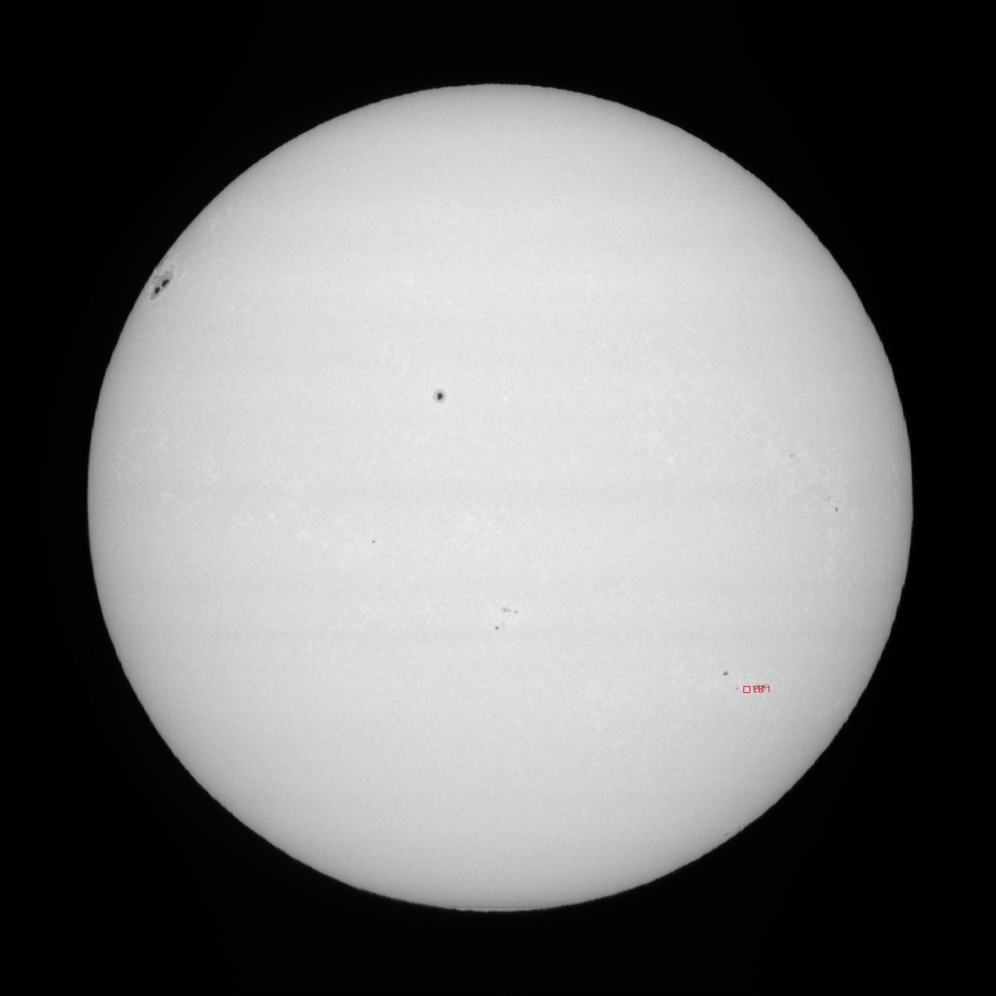
And for each bomb, it will create an image which shows the region of the spectrum which is used to detect the bomb. This is for example what is automatically generated for the bomb described above:

Algorithm details

Note	This is a description of the algorithm that I implemented in an adhoc fashion: I’m not a mathematician nor a scientist: I’m an engineer and the algorithm above was implemented using my "intuition" of what I thought would work. It is likely to change as new versions are released.

The algorithm is based on the following steps:

for each frame in the SER file, identify the "borders" of the sun
perform a Gaussian blur on the spectrum to reduce noise
within the borders, compute, for each column, the average intensity of the spectrum for the center of the line and the wings separately. The center of the line is defined as the range [-0.35Å, 0.35Å] and the wings as the range [-5Å, -0.35Å[ ∪ ]0.35Å, 5Å]
compute the maximum intensity of the wings, starting from the center of the line, and going outwards until we reach the maximum intensity (local extremum)
compute the average of each column average intensity for the wings (the "global average")

With Ellerman bomb scoring parameters defined below, the algorithm proceeds per column:

For each column index x in the spectrum image:
Build a neighborhood of up to 16 columns around x: Nₓ = { x + k | k ∈ ℤ, |k| ≤ 8 }, clamped to the image boundaries.
Compute the overall mean column intensity Ī_global = (1 / N_total) ∑_{j=1..N_total} Ī(j).
Exclude any columns in Nₓ whose average intensity falls below 90 % of Ī_global, since very dark columns (usually sunspots) would pull down our estimate of the local wing background and hide true brightening events. Call the remaining set Mₓ and let m = |Mₓ|.
If m < 1, there aren’t enough valid neighbors to form a reliable background—skip column x.
On the Gaussian-smoothed data, measure three key values at column x:
c₀ ≔ I_center(x), the mean intensity in the core region of the spectral line.
c_w ≔ I_wing(x), the average intensity across the two wing windows at ±1 Å.
c_max ≔ max_{p ∈ wing-pixels nearest ±1 Å} I(p, x), the single highest wing intensity near the expected shift.
Compute the local wing background r₀ = (1 / (m−1)) ∑_{j ∈ Mₓ, j≠x} I_wing(j). Using only nearby “bright enough” columns keeps the background estimate from being skewed by dark features.
Define a line-brightening factor B = max(1, c₀ / min(r₀, I_center,global)). Ellerman bombs boost the wings without greatly brightening the core, whereas flares brighten both.
Form an initial score S₀ = 1 + c_max / min(r₀, I_wing,global), where I_wing,global = (1/N_total) ∑_{j=1..N_total} I_wing(j). This compares the local wing peak to the typical wing level across the image.
Adjust for how many neighbors were used: S₁ = S₀ × (m / 16). Fewer valid neighbors mean less confidence, so the score is scaled down proportionally.
Compute the wing-to-background ratio rᵢ = c_max / r₀. If rᵢ ≤ 1.05, the wing peak is too close to the local background and the column is discarded. Otherwise, we boost the score further:
Raise S₁ to the power of e^{rᵢ}, giving S₂ = S₁^( e^{rᵢ} ). This makes the score grow quickly when the wing peak stands out strongly.
Multiply by √(c_max / c₀) to get S₃ = S₂ · √(c_max / c₀). That emphasizes cases where the wings are much brighter than the core.
Finally, penalize any shift away from the ideal ±1 Å wing position. If y_core and y_max are the pixel locations of line center and wing peak, compute Δλ = |y_max – y_core| × (Å / pixel), then S_final = S₃ / (1 + |1 Å – Δλ|).
If S_final > 12, mark column x as a candidate event. Use the value of B to decide:
When B < 1.5, it behaves like an Ellerman bomb (wings bright, core unchanged).
When B > 2, it matches a flare (both core and wings bright).
If 1.5 ≤ B ≤ 2, the result is ambiguous and ignored.

All thresholds (0.9× global mean, 1.05 ratio, score > 12, B cutoffs) were chosen by testing on data and visually inspecting results.

Post-filtering

There will often be cases where the same bomb is detected in multiple frames. Therefore, we need to do some merging of bombs which are spatially connected.

Eventually, we apply a limit threshold: if there are more than 5 Ellerman Bombs detected in an image, then we consider the detection to be false positives (this happens typically on saturated images, or images with too much noise). This is a bit arbitrary, but it seems to work well in practice.

Test data

I had about ~1100 scans I could reuse for detection, and it successfully discovered Ellerman bombs candidates in about 10% of them. Of course this required some tuning and several runs to get the parameters right. This doesn’t mean that you have 10% chances of finding an Ellerman bomb in your data, because the test data I have is biased (I often do 10 to 20 scans in a row, within a few minutes, to perform stacking, so if a bomb is detected in an image, it has decent chances of being detected in the next one). Also, I am using the term "Ellerman Bomb candidate", because there’s nothing better than visual confirmation to make sure that what you see is indeed an Ellerman bomb: an algorithm is not perfect, and it may fail for many reasons (noise, saturation, artifacts, etc.)

Here are a few examples of Ellerman bombs candidates detected in my data:

Conclusion

This blog post described my first visual Ellerman bomb detection. Then I described how I implemented an algorithm to automatically detect Ellerman bombs in JSol’Ex 3.2. I am very happy to release this to the wild, so that this kind of discovery is made more accessible to everyone. Of course, as I always say, you should take the detections with care, and always review the results. This is why you get both a global "map" of the detected bombs, and a detailed view of each bomb, which can be used to confirm the detection. In addition, I recommend that you create animations of the regions, which you can simply do in JSol’Ex by CTLR+clicking on the image then selecting an area around the bomb.

Finally, I’d like to thank my friends of the Astro Club de Challans, who heard me talk about Ellerman bombs detection for a while, showing them preliminary results, and who were very supportive of my work. Last but not least, thanks again to my wife for her patience, seeing me work on this (too) late at night!

Ellerman Bombs Detection with JSol’Ex 3.2