
Measuring the Sun’s oscillations with an amateur spectroheliograph
22 September 2026
Tags: solex jsolex shg700 solar astronomy doppler helioseismology
|
Note
|
This is an English version of my blog post originally written in French, published on 16 September and updated on 19 September. It includes the corrected results, and a new section about weighing the Sun. |
The Sun has a beating heart. What if we could hear it?[1]
In this post, I am going to tell you how I measured the Sun’s five-minute oscillations with a 102 mm refractor costing €250 and a spectroheliograph (SHG 700), from my garden. These oscillations are the basis of helioseismology, the discipline which probes the interior of the Sun the way a seismologist probes the interior of the Earth. Looking for an original experiment to complete my upcoming talk at the Rencontres du Ciel et de l’Espace in Paris, I suspected it would be possible, but I did not know whether I would succeed.
In the end, I recovered six resonance "modes" of the Sun (I learnt the word mode while doing this experiment), and their frequencies agree admirably[2] with the values published by the SOHO satellite.
Having found no reference to this kind of velocity measurement made by an amateur, which does not mean none exists, I believe this is a world first. Measurements based on the brightness of the surface do exist, I come back to this below.
This post focuses on the results and on the experiment itself. If you are interested in the method and the analysis, I refer you to the complete article I wrote on the subject, available as a PDF in English and a PDF in French.
The five-minute oscillations
In 1962, Leighton, Noyes and Simon discovered that the surface of the Sun oscillates, with a period of about five minutes. Ulrich explained it in 1970: these are sound waves, produced by convection below the surface, which bounce between the deep layers and the photosphere, and end up resonating.
In a resonating cavity, not every note is allowed: an organ pipe produces a fundamental and its harmonics, and nothing in between. The Sun does the same, but two numbers are needed to describe one of its notes: the size of the wave at the surface, and its frequency. If you sort all the motions of the surface by these two criteria, the power is not spread at random: it concentrates along narrow lines, called ridges.
Seeing these ridges is seeing the Sun resonate. Deubner observed them for the first time in 1975, and he could distinguish three or four of them. This is what I wanted to try to reproduce.
|
Note
|
A personal aside: when I started my studies in 1998, I wanted to do astrophysics, and I gave up when I saw the level of mathematics required (I had already talked about this here). For this exercise, I relied on my experience developing JSol’Ex and on my many observations to establish the protocol. Reading the papers allowed me to understand the steps needed to obtain the diagram, but the understanding of the equations and models essentially escaped me. Without the help of AI, I could never have done this experiment or analysed the results correctly. This reflects my complicated relationship with AI, which would deserve a post of its own: it will surprise no one that I am terrified by the speed at which AI is changing our lives, with undeniable ethical, social, societal and environmental implications, but I am also fascinated by what it makes possible, and the result of this post is an example. For me, the question is really not whether AI works or not: it works, and it is impressive. The benefit/risk question, and the question of prioritising AI development over environmental issues in particular, are the points we should be discussing. In short, I curse it as much as I admire it. I live the contradictions of this relationship every day, and I do not yet know how to handle them: until proven otherwise, I remain a fallible human being, and I reassure myself by telling myself that what I am doing here is science, something useful, unlike the adverts blooming everywhere, or the AI-generated videos and music we see at French tech conferences… but I digress. |
The experiment
The protocol is, in the end, fairly simple: one scan of the disc every minute, for six hours, without interruption, in an iron line whose Landé factor (which represents the sensitivity to magnetic fields) is as close to zero as possible. This gives 336 retained scans and 1.4 TB of video, that is a movie of the Sun at one frame per minute, in which every pixel contains a line profile. I had to discard a few scans for various reasons (geometry, artefacts, mount resonance, and so on) but the bulk is there.
A spectroheliograph, such as Christian Buil’s Sol’Ex or the SHG 700 I use, does not directly produce an image of the Sun. At every point of the disc, it records the complete profile of a spectral line, and this is the whole difference with a filter: a filter gives an intensity, a spectroheliograph gives the exact position of the line, which can be converted directly into a velocity (Doppler effect).
Figure 1. One of my scans, in the neutral iron line at 5434.5 Å
Let us now talk about what is probably the most surprising point, if you only look at the numbers: what we are trying to measure is much finer than the nominal resolution of the instrument. So there is a trick. On my spectrum, one pixel corresponds to 5,737 m/s, whereas the oscillations I am looking for are a few hundred metres per second: a velocity of 300 m/s shifts the line by a twentieth of a pixel. How can one reach a precision of a twentieth of a pixel? In practice, it can be inferred, by comparing each point of the disc with itself rather than with a model. It is the same kind of problem as the differential rotation measurement I wrote about, but far more demanding.
Once the velocities are measured, what remains is to sort the motions by size and frequency, and to look at where the power is.
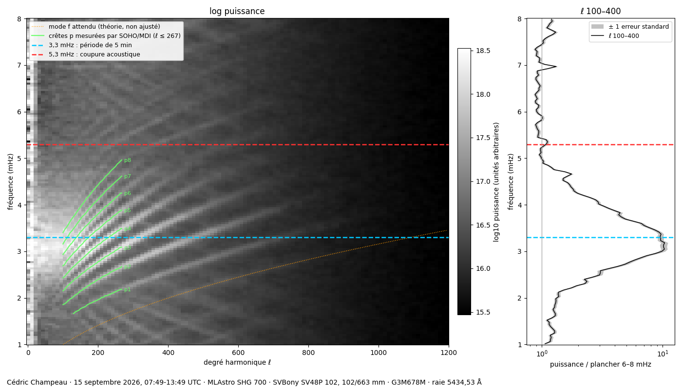
Figure 2. The resonance ridges of the Sun, seen from my garden
One can clearly see "curves" brighter than the background: these are the famous resonance ridges of the Sun. The horizontal axis measures the size of the waves: the further right, the smaller the structures. The vertical axis is the frequency, knowing that 3 mHz corresponds to one oscillation every 5 minutes 33 seconds. The green curves are not a fit: they are the ridges measured by the SOHO satellite, laid as they are on my diagram.
The comparison with SOHO
Seeing lines is one thing, making sure they are the right ones is another, and this is what took me the most work: however nice the diagram, how can one make sure that the resonance modes of the Sun have really been found, and that the results are not a hallucination?
The frequencies of the solar modes are published: the SOHO/MDI project makes available, on the Stanford servers, the tables fitted on its own spectra. So I compared my six ridges with the published values:
| Ridge | MDI table (mHz) | My measurement (mHz) | Difference |
|---|---|---|---|
p1 |
1.6441 |
1.653 |
+9 µHz |
p2 |
2.0072 |
2.023 |
+16 µHz |
p3 |
2.3404 |
2.329 |
−12 µHz |
p4 |
2.6356 |
2.636 |
0 µHz |
p5 |
2.9201 |
2.926 |
+6 µHz |
p6 |
3.1902 |
3.181 |
−9 µHz |
The mean difference is 9 µHz, a fifth of the resolution of my series.
What matters in this table is that no parameter is adjusted. The frequency scale comes solely from the time stamps written in the SER files, the size scale solely from the radius of the disc measured in pixels. The two measurements (time and pixels) are subject to independent uncertainties, and they agree nonetheless.
The mount problem
I expected the limit of the exercise to come from the seeing, which was poor during all my observations (clear sky, but definite turbulence). In reality, the chart showed surprising ridges which are not part of the SOHO results. The cause? The mount!
My SAL-33 uses harmonic drives, which have a periodic error of 430 seconds, of about 16 arc seconds peak to peak (Minh Nguyen, of ML Astro, confirmed it when I sent him my measurements). During the fifteen seconds a scan lasts, this error changes the speed at which the image moves across the slit, and what remains is a distortion which shifts the content of the image by a few pixels, differently from one scan to the next. In other words, my successive velocity maps are slightly shifted with respect to each other, which blurs the ridges. I must say that not only had I not anticipated this problem, but I would never have believed that the diagram would reveal this flaw and that its amplitude could be measured!
So I measured this slip, and corrected it. The contrast of the oscillations increases by nearly half, the frequencies do not move, and their agreement with SOHO improves a little more: the largest difference drops from 19 to 16 µHz.
Since this kind of correction can easily turn into an illusion (you look for something, you end up finding it), I applied exactly the same correction to randomly drawn scans. If my method improved things by mere mathematical construction, this control would have improved too. It gets worse instead.
The case of the f mode
There remains a separate family of waves, the f mode, which is not a sound wave but a surface wave, comparable to waves on water. Its theoretical position is the orange curve of the diagram. It is much fainter than the other ridges, but it is there: for the smallest waves (beyond degree 450), a ridge follows the theoretical curve to within 1 %.
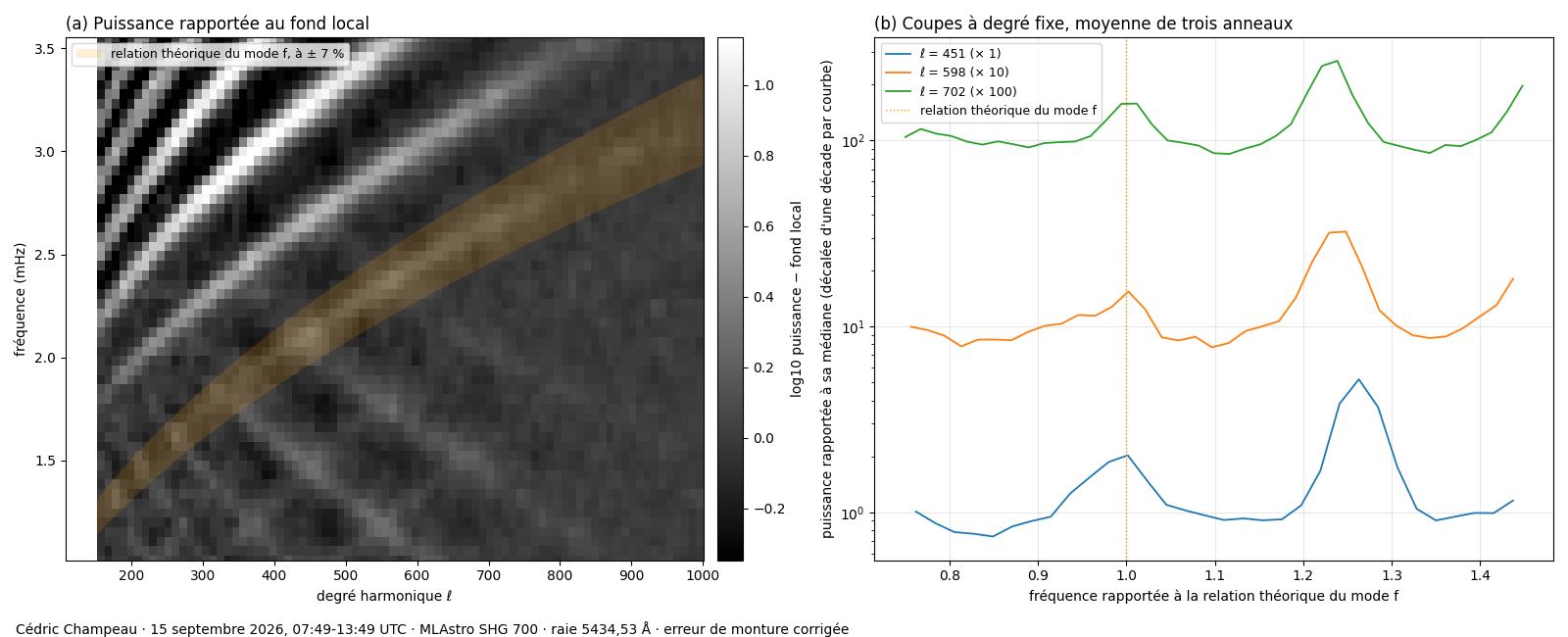
Figure 3. The f-mode region: the ridge follows the theoretical position, in orange
Below degree 400, it is too faint for me to detect. This figure also shows lines running down at an angle: they are leftovers of the mount flaw, which my correction does not remove completely.
Bonus: weighing the Sun
Since the f mode is a surface wave, like a swell on the ocean, it obeys a very simple relation between its rhythm, its length and gravity: the stronger the gravity, the faster the wave oscillates. A fisherman who times the swell and measures its length can deduce the gravity of the Earth.
Good news, my diagram gives me exactly these two pieces of information: how fast the waves oscillate, and how many of them fit around the Sun (this is what the "degree" measures). Newton tells us that the gravity of a body depends on its mass and its radius. Combining the two, the radius cancels out and what remains is the mean density of the Sun. The whole computation fits on one page:
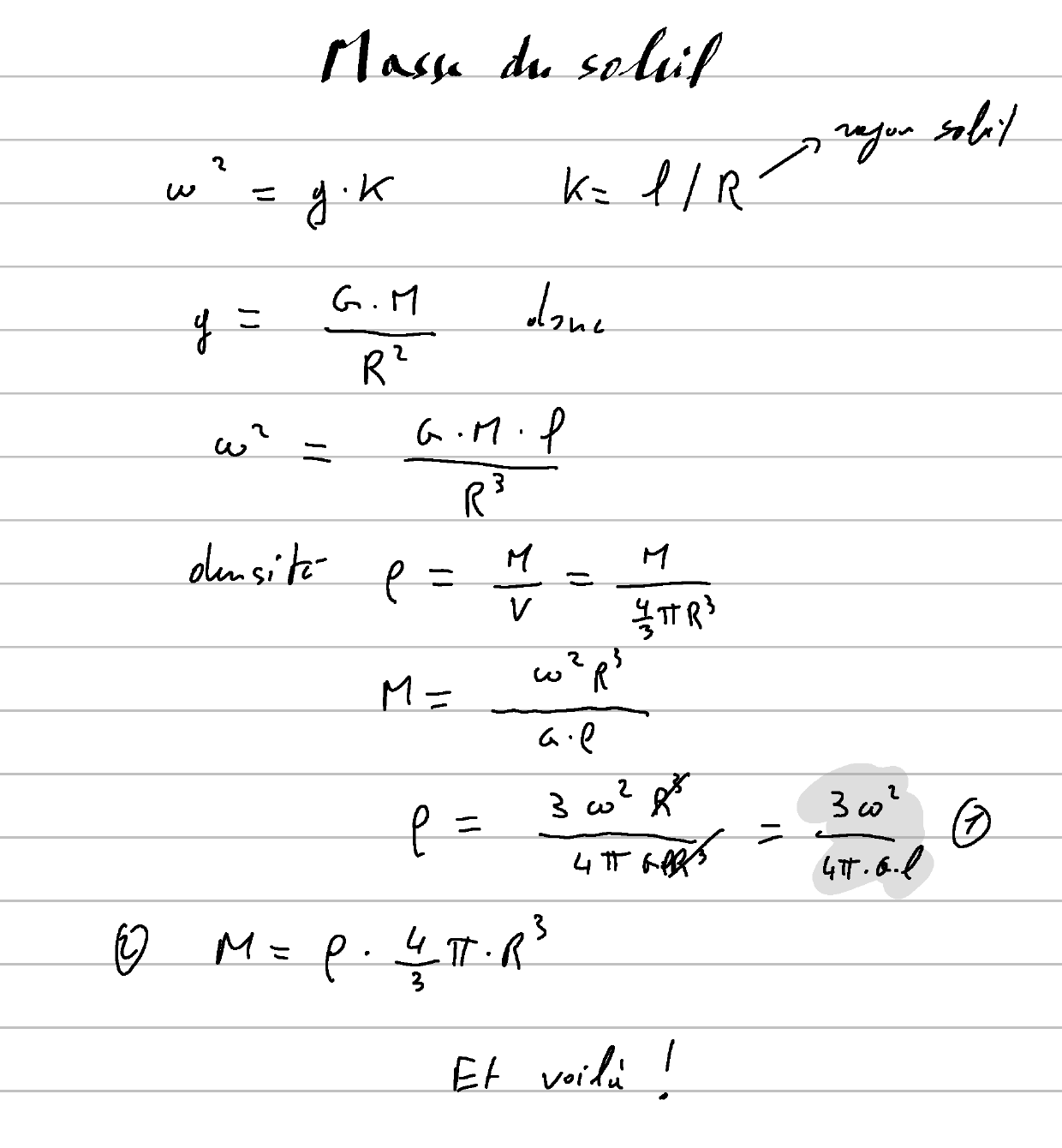
Figure 4. Density of the Sun from the f mode, on one page
For each wave, I read its rhythm and its degree on my diagram, and the formula gives the density. For instance, at degree 650, one oscillation every 6 min 33 s gives 1,406 kg/m³. Over ten waves, the average is 1,410 kg/m³, for 1,408 in the literature. It is a mean value, barely more than water: the centre is 150 times denser, and the surface thousands of times less dense than air.
One step remains. To compute the mass, the volume is needed, hence the radius, estimated at 695,700 km. This gives 1.989 x 10³⁰ kg, for a commonly accepted value of 1.988 x 10³⁰ kg.
One has to stay modest: there are measurement errors and approximations, so it is partly by luck that I land so close to the reference value. Still, I love physics!
The mistake in the first version
The first version of this post, published on 16 September, told a different story about the f mode. I could not find it where it belonged, but I saw a band of power 4 to 8 % lower, present in my three sessions, which I could not explain. I ended by saying that if anyone had an idea, I was interested.

Figure 5. The diagram of the first version: the ridges are split

Figure 6. The band I took for an unknown feature
After publication, I received on the Cloudy Nights forum two remarks from Matt Penn, who spent thirty years doing solar physics in several American observatories, and who is behind the Citizen CATE and DEB citizen science eclipse experiments.
The first concerns my "world first". Measurements of these oscillations had already been made with amateur equipment, and by himself: in 2020, with a 60 mm refractor, he already obtained a diagram of the same kind. Those measurements are based on the brightness variations of the surface, not on velocities, which is simpler to obtain. My first therefore only concerns the velocity measurement.
The second remark was more embarrassing: on my diagram, every ridge seemed to be split in two, which is not normal. His advice was to find the cause of this splitting before trying to explain the band below the f mode.
While searching, I found a mistake in my drift computation. To analyse the same region of the Sun for six hours, my script moves the analysed area to compensate for the rotation of the Sun. Because of this mistake, the area did not follow the surface exactly, and the surface was slipping across my analysed area at 1.5 km/s.
Now, a slip shifts the apparent frequency of the waves: upwards for those travelling one way, downwards for those travelling the other way. Every ridge splits in two, and my mysterious band was nothing but the lower half of the f mode. Professionals actually use this effect to measure the flows below the surface of the Sun.
Once the tracking was fixed, the ridges became single and sharper again, the f mode appeared where it belongs, and the mean difference with the SOHO tables went from 11 to 9 µHz. The script is fixed, and it now checks by itself that the analysed area follows the surface.
Many thanks to Matt Penn for his remarks.
In practice
Everything happens in JSol’Ex, in a single batch: the software reconstructs the images, fits the disc, corrects the geometry, then runs my Python script in its embedded interpreter, which computes the velocities, the spectrum and the figures. By the way, thank you GraalVM! There is no other software in the chain, and for me this is the important point, the one that makes me spend time developing JSol’Ex: making this kind of measurement accessible to as many people as possible. However, my Python scripts use NumPy, which means that, given the limits of GraalVM, the script will not work on Windows.
Processing the 354 files, diagram included, takes about 2 h 30 on a Ryzen 9 9950X. Think about it: nearly 1.5 TB of data processed in 2 h 30 with these charts produced directly! I do not know the context of Deubner’s experiment, but I suppose the processing must have taken much longer back then.
The rest is patience: six hours of uninterrupted tracking, a well-chosen line, and a sky willing to stay clear. Fortunately, the acquisition itself is fully automated, and all I had to do was watch the weather and the sky.
Conclusion
What makes this result possible is not the equipment, which is fairly ordinary in the end: a 102 mm refractor, a commercial spectroheliograph (a Sol’Ex should work too, preferably with a thinner second-generation slit) and a light mount. No, it is rather perseverance (the combination of a long regular series and somewhat lengthy processing) and, I am tempted to say, the simplicity of implementing the processing in JSol’Ex.
It is also, to my dismay, the use of generative AI, which allowed me to get past the mathematical formalism to understand the intent of the equations and models, and to write the code which computes the velocities and the diagram.
As always with what I write here, take it with the necessary caution: I am not a solar physicist, I am not a scientist, and I have most probably made approximations I should not have made. This is precisely why I publish the complete article at the same time as this post: the numbers, the uncertainties and the limitations are detailed there, and everything can be checked. I did check everything where I have the skills, in particular the code, and what reassures me is that I did have to correct AI mistakes throughout the development: humans still have a say (for how long?).
In short, if you have a spectroheliograph and a mount which tracks properly for a few hours, you can redo this measurement, and I would very much like to see your results.
Going further
1. A knowledgeable reader would tell me that these are not heartbeats and that we cannot hear them. A better metaphor would be a ringing bell, but poetry sometimes has to depart from scientific rigour.
2. This is the amateur speaking. For actual numbers, trust the paper.
