TamboUI (pronounced like the french word “tambouille”, slang for "cooking up something" or "makeshift creation") was born a bit by accident: a couple months ago, Cédric was asking about which TUI libraries that tools like Claude Code were using. Max Andersen answered that most likely this was Ratatui, a framework written in Rust. Both thought that it was a bit sad that there was no such library for Java.

A few weeks later, Cédric did an experiment by asking AI (Claude Code) to port Ratatui to Java. The result was fairly impressive, and the beginning of a collaboration that led to the creation of TamboUI. In fact, Max gave you a hint last year that this was going to happen.

That said, TamboUI is not a Ratatui port nor is it a Textual port. We’ve put a lot of effort in going beyond the initial AI generated port. The library was designed with Java developers in mind, inspired by the good things found in other ecosystems’ approach to TUI frameworks. It offers a multi-layer API: from low-level widget primitives (like Ratatui), to a managed TUI layer with event handling, up to a declarative Toolkit DSL that handles the event loop and rendering thread for you—things that Ratatui doesn’t really cover. This brings the power of Ratatui, Textual or Rich to the Java ecosystem, with the Java touch!

Not only that, TamboUI is also GraalVM native compatible! This means that you can compile your Java TUI applications as native binaries, making Java a first class citizen in terminal applications development, with low memory footprints and fast startup!

If you want to give it a try, the easiest is to run our demos using JBang:

At this stage, the APIs are still unstable and subject to change. TamboUI is developed with the mindset of being framework-agnostic and having as few external dependencies as possible. You can choose between several backends like JLine, Aesh or the built-in Panama backend. By choosing the latter, you’ll get the best performance while not depending on any external library.

Whether you want to build:

Give TamboUI a try and let us know what worked and what could be improved!

Check out the documentation at https://tamboui.dev/docs/main/, join us on Zulip, or browse the source on GitHub. We’d love your feedback and contributions!

We would like to thank the following people for their ideas, suggestions and contributions to the creation of first public release of TamboUI (in alphabetical order):

and of course to the Ratatui and Textual creators for their inspiration and work.

L’un des aspects fascinants du Soleil est qu’il ne tourne pas comme un corps solide. Contrairement à la Terre, qui effectue une rotation en 24 heures quelle que soit la latitude, la vitesse de rotation du Soleil varie avec la latitude : l’équateur tourne plus vite que les pôles. Ce phénomène, appelé rotation différentielle, est étudié depuis le 19ème siècle et reste un sujet de recherche important en physique solaire.

Les régions équatoriales du Soleil effectuent une rotation en environ 25 jours, tandis que près des pôles, cela prend environ 35 jours. Cette rotation différentielle joue un rôle clé dans le mécanisme de dynamo solaire qui génère le champ magnétique du Soleil et pilote le cycle solaire de 11 ans.

Dans cet article, je vais expliquer comment j’ai ajouté une fonctionnalité dans JSol’Ex 4.5.0 qui permet aux astronomes amateurs de mesurer cette rotation différentielle directement à partir d’un scan obtenu avec un spectrohéliographe. Une erreur fréquente est de penser que cette mesure n’est pas possible parce que la dispersion spectrale d’un spectrographe comme le Sol’Ex est typiquement d’environ 0.1 à 0.2 Å, c’est-à-dire plus grand que l’échelle de ce que nous essayons de mesurer (2 km/s, soit environ 0.04 Å). En pratique, nous devrons obtenir une précision sub-pixellaire et cet article explique comment y arriver.

Le principe derrière la mesure est simple : l'effet Doppler. Quand une source lumineuse se déplace vers nous, la longueur d’onde est décalée vers le bleu du spectre (blueshift). Quand elle s’éloigne, la longueur d’onde se décale vers le rouge (redshift).

Puisque le Soleil tourne, un limbe se déplace toujours vers nous (le limbe Est) tandis que l’autre s’éloigne (le limbe Ouest). En mesurant le décalage de longueur d’onde d’une raie spectrale aux deux limbes, nous pouvons calculer la vitesse de rotation.

On pourrait se demander ce qu’il en est du mouvement propre de la Terre : nous orbitons autour du Soleil à environ 30 km/s, ce qui est bien plus grand que la vitesse de rotation solaire d’environ 2 km/s que nous essayons de mesurer. Ce mouvement orbital produit effectivement un décalage Doppler de tout le spectre solaire. Cependant, cet effet s’applique de manière égale à tous les points que nous pouvons mesurer : en d’autres termes, puisque tout le spectre est décalé de manière uniforme, tout s’annule. Il en va de même pour toute vitesse radiale du Soleil par rapport à la Terre (qui varie légèrement tout au long de l’année car l’orbite de la Terre est elliptique).

La formule fondamentale reliant le décalage Doppler à la vitesse est :

Où :

L’un des aspects les plus délicats de cette implémentation est de transformer correctement les coordonnées que nous manipulons. L’algorithme commence avec les coordonnées héliographiques (où nous voulons mesurer) et les transforme en coordonnées des trames SER originales (où les données spectrales se trouvent).

1. Coordonnées héliographiques (point de départ)

Nous commençons par spécifier des points en coordonnées héliographiques :

Cela nécessite deux paramètres solaires calculés à partir de la date d’observation :

2. Coordonnées image

Les coordonnées héliographiques sont converties en positions de pixels dans l’image reconstruite. Cela implique d’inverser les corrections appliquées pendant la reconstruction :

3. Coordonnées du fichier SER (destination)

Finalement, les coordonnées image sont mappées vers le fichier vidéo SER brut :

Ce mapping inverse nous permet d’extraire le profil spectral exact à n’importe quelle position héliographique.

Les mesures brutes sont bruitées. Pour produire une courbe de rotation propre, JSol’Ex utilise un pipeline de traitement en deux étapes :

La forme standard de la loi de rotation différentielle (aussi connue comme la formule de Faye, même si la formule originale n’incluait pas le 3ème terme) est :

Où :

JSol’Ex compare les résultats mesurés avec les coefficients largement utilisés de Snodgrass & Ulrich (1990) :

Cela donne une période de rotation équatoriale d’environ 24.5 jours et une période polaire d’environ 34 jours. Convertie en vitesse linéaire à la surface solaire (rayon ≈ 696 000 km), la vitesse de rotation équatoriale est d’environ 2.0 km/s.

JSol’Ex ajuste également ses propres coefficients A, B, C à partir de vos mesures, permettant une comparaison directe avec les valeurs de référence.

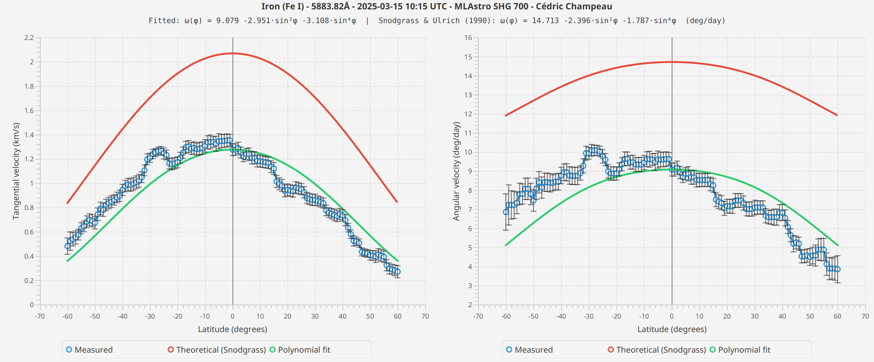
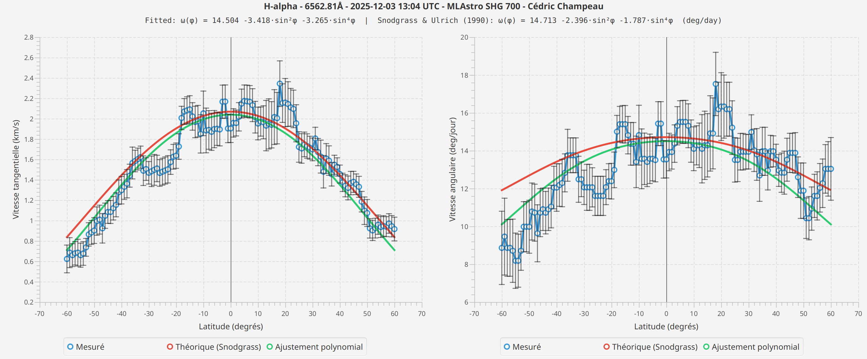
Ci-dessous des exemples de profils de rotation différentielle mesurés avec JSol’Ex en utilisant deux raies spectrales différentes. Ces mesures ont été prises à des dates différentes avec des conditions de seeing différentes.

La qualité des résultats dépend fortement du seeing atmosphérique. Un mauvais seeing floute les raies spectrales et rend la détermination précise du centre difficile. Les meilleurs résultats sont obtenus avec d’excellentes conditions de seeing et un instrument bien focalisé. Enfin et surtout, une haute résolution spectrale est préférée, ce qui est normalement le cas avec le Sol’Ex (HR) ou le SHG 700.

Vous pouvez aussi vous demander quelle raie spectrale vous devriez observer. J’ai testé l’algorithme avec Fe I, Na D2 et H-alpha, donnant les résultats ci-dessous. En pratique, les raies d’absorption fortes devraient en théorie produire les meilleurs résultats, car :

Les raies très larges comme Ca II K sont trop larges pour un ajustement de Voigt précis et produiront des résultats peu fiables. Les raies trop étroites peuvent aussi représenter un défi pour l’ajustement de Voigt mais peuvent fonctionner aussi.

Mesurer la rotation différentielle avec du matériel amateur aurait semblé impossible il y a quelques années seulement. Des pionniers comme Peter Zetner ou Christian Buil nous ont montré la voie. Ce que j’essaie de faire, comme toujours avec JSol’Ex, c’est de rendre ceci accessible à encore plus de personnes au prix de la "magie", c’est-à-dire que certaines personnes partageront très probablement des résultats sans comprendre la science derrière. Je ne suis pas trop inquiet par cela, parce que je suis moi-même passé par là : apprécier la reconstruction d’images SHG, puis comprendre comment ça fonctionne, puis me poser des questions comme "pourquoi est-il même possible de mesurer des vitesses Doppler si petites ?" : c’est une construction intellectuelle qui prend du temps. Nous, membres de la communauté Sol’Ex, pouvons faire mieux, je pense, pour apporter cela aux masses, en partageant nos idées et en écrivant des logiciels comme celui-ci.

Cette fonctionnalité rejoint la liste croissante des capacités scientifiques dans JSol’Ex : détection des bombes d’Ellerman, identification des régions actives, et maintenant mesure de la rotation différentielle. Chacune de celles-ci met des analyses de niveau professionnel à la portée des astronomes amateurs, mais, comme toujours, soyez prudent avec ce que je dis : je ne suis pas un scientifique, juste un ingénieur. Je n’ai aucun doute que j’ai fait des approximations, ou pris des libertés que je n’aurais probablement pas dû prendre.

One fascinating aspect of the Sun is that it doesn’t rotate like a solid body. Unlike the Earth, which completes one rotation in 24 hours regardless of latitude, the Sun’s rotation rate varies with latitude: the equator rotates faster than the poles. This phenomenon, called differential rotation, has been studied since the 19th century and remains an important research topic in solar physics.

The equatorial regions of the Sun complete a rotation in approximately 25 days, while near the poles, it takes about 35 days. This differential rotation is thought to play a key role in the solar dynamo mechanism that generates the Sun’s magnetic field and drives the 11-year solar cycle.

In this blog post, I will explain how I implemented a feature in JSol’Ex 4.5.0 that allows amateur astronomers to measure this differential rotation directly from their spectroheliograph data. A common mistake is to think that this measurement is not possible because the spectral dispersion of a SHG like the Sol’Ex is typically around 0.1 to 0.2Å, which larger than the scale of what we’re trying to measure (2 km/s, which is about 0.04Å). In fact, what we are trying to measure requires sub-pixel precision and we can achieve that.

The principle behind the measurement is simple: the Doppler effect. When a light source moves towards us, the wavelength is shifted towards the blue end of the spectrum (blueshift). When it moves away, the wavelength shifts towards the red (redshift).

Since the Sun rotates, one limb is always moving towards us (let’s say the East limb) while the other is moving away (the West limb). By measuring the wavelength shift of a spectral line at both limbs, we can calculate the rotation velocity.

One might wonder about the Earth’s own motion: we orbit the Sun at approximately 30 km/s, which is much larger than the ~2 km/s solar rotation velocity we’re trying to measure. This orbital motion does produce a Doppler shift of the entire solar spectrum. However, this affects equally all points we can measure: this is a global shift which affects all measurements equally and cancels out. The same is true for any radial velocity of the Sun relative to the Earth (which varies slightly throughout the year as Earth’s orbit is elliptical).

The fundamental formula relating Doppler shift to velocity is:

Where:

One of the trickier aspects of this implementation is correctly mapping between the different coordinate systems involved. The algorithm starts with heliographic coordinates (where we want to measure) and maps them back to the original SER frames (where the spectral data lives).

1. Heliographic Coordinates (starting point)

We begin by specifying points in heliographic coordinates:

This requires two solar parameters computed from the observation date:

2. Image Coordinates

The heliographic coordinates are converted to pixel positions in the reconstructed image. This involves reversing the corrections applied during reconstruction:

3. SER File Coordinates (destination)

Finally, the image coordinates are mapped to the raw SER video file:

This reverse mapping allows us to extract the exact spectral profile at any heliographic location.

The raw measurements are noisy. To produce a clean rotation curve, JSol’Ex uses a two-stage processing pipeline:

The standard form of the differential rotation law (also known as the Faye formula, even if the original formula didn’t include the 3rd term) is:

Where:

JSol’Ex compares measured results with the widely-used coefficients from Snodgrass & Ulrich (1990):

This gives an equatorial rotation period of about 24.5 days and a polar period of about 34 days. Converting to linear velocity at the solar surface (radius ≈ 696,000 km), the equatorial rotation velocity is approximately 2.0 km/s.

JSol’Ex also fits its own A, B, C coefficients from your measurements, allowing direct comparison with the reference values.

Below are example differential rotation profiles measured with JSol’Ex using two different spectral lines. These measurements were taken on different dates with different seeing conditions.

The quality of results depends heavily on atmospheric seeing. Poor seeing blurs the spectral lines and makes accurate center determination difficult. Best results are obtained with excellent seeing conditions and a well-focused instrument. Last but not least, a high spectral resolution is preferred, which is normally the case with Sol’Ex (HR) or the SHG 700.

You may also wonder which spectral line you should observe. I tested the algorithm with Fe I, Na D2 and H-alpha, giving the results below. In practice, strong absorption lines should in theory produce the best results, because:

Very broad lines like Ca II K are too wide for accurate Voigt fitting and will produce unreliable results. Too narrow lines may also represent a challenge for Voigt fitting but may work too.

Measuring differential rotation with amateur equipment would have seemed impossible just a few years ago. Pioneers like Peter Zetner or Christian Buil showed us the path. What I’m trying to do, as always with JSol’Ex, is to make this accessible to even more people at the cost of "magic", which is that some people will very likely share results without understanding the science behind it. I’m not too concerned by this, as I, myself, have been going this way: enjoying SHG image reconstruction, then figuring out how it works, then asking myself questions like "why is it even possible that we measure Doppler velocities so small?": this is an intellectual construct that takes time and we can do better, I think, at brining this to the masses, sharing our insights.

This feature joins the growing list of scientific capabilities in JSol’Ex: Ellerman bomb detection, active region identification, and now differential rotation measurement. Each of these brings professional-level analysis within reach of amateur astronomers, but, as always, be cautious with what I’m saying: I’m not a scientist, just an engineer. I have no doubts that I made approximations, or took liberties that I should probably not have taken.

However, I do think that this brings value to the ecosystem.

Nous voici 2 ans et demi plus tard, JSol’Ex arrive en version 4. Entre temps, le nombre d’utilisateurs a explosé et mon logiciel est exploité non seulement par les utilisateurs du Sol’Ex de Christian Buil, mais aussi pour des spectrohéliographes commerciaux comme le MLAstro SHG 700 (que j’utilise désormais). JSol’Ex a apporté de nombreuses innovations, comme la possibilité d’exécuter des scripts pour générer des animations, faire du stacking, créer des images personnalisées, ou encore la détection automatique d’éruptions, des régions actives (avec annotation), la détection de bombes d’Ellerman, la correction des bords dentelés et j’en passe.

Récemment, JSol’Ex a été utilisé pour réaliser un Atlas de Spectrohéliogrammes, et mentionné dans un article précisément sur la détection des bombes d’Ellerman. Bref, JSol’Ex était devenu suffisamment mature pour faire de la "vraie science", chose qui m’a toujours un peu effrayé pour être honnête.

Ainsi, j’ai toujours refusé d’intégrer une fonctionnalité dans JSol’Ex, qui m’a pourtant été demandée de nombreuses fois : la possibilité de l’utiliser pour soumettre des images dans la base de données BASS2000 de l’Observatoire de Paris-Meudon. Plusieurs raisons à cela : d’une, je ne faisais pas confiance à mon propre logiciel pour sa qualité "scientifique". Si je le savais capable de produire de "belles images", il est tout à fait différent de s’en servir pour une exploitation scientifique. D’autre part, il n’était pas question pour moi d’intégrer une fonctionnalité qui avait été développée par Valérie Desnoux (autrice de INTI) et l’équipe de Meudon sans son accord, par respect pour son travail.

Cependant, vous aurez compris que les temps ont changé et que la pression des utilisateurs ainsi que mes discussions avec Florence Cornu, du projet SOLAP, aux Rencontres du Ciel et de l’Espace fin 2024, puis aux JASON en Juin dernier ont eu raison de mes doutes. Avec son accord et celui de Valérie, je suis donc heureux de vous annoncer que JSol’Ex 4 est officiellement supporté pour soumettre vos images dans la base de données BASS 2000 !

Ne souhaitant pas faire les choses à moitié, j’ai particulièrement peaufiné le logiciel pour simplifier cette procédure. J’ai souhaité faire les choses avec sérieux, puisqu’il s’agit d’une base de données professionnelle, exploitée par des scientifiques. Ainsi, une chose importante pour moi était de guider l’utilisateur dans ce processus et de lui faire comprendre l’importance de la qualité des données, tout en simplifiant le processus de soumission.

Ainsi par exemple, BASS2000 n’a que très peu de tolérance sur les problèmes d’orientation de l’image : il faut que le Nord solaire soit à moins de 1 degré d’erreur, sinon l’image sera refusée. L’assistant intègre donc un outil pour aider à vérifier l’orientation et corriger les erreurs minimes dues par exemple à une mise en station imparfaite.

L’assistant guidera aussi l’utilisateur dans son processus de soumission, en lui demandant de bien vérifier toutes les métadonnées associées à l’observation, et ira jusqu’à envoyer l’image sur le serveur FTP de BASS2000 pour validation par les équipes.

Je suis particulièrement reconnaissant à Florence CORNU pour son aide afin que les images JSol’Ex soient acceptées dans la base et je remercie mes beta-testeurs qui ont patiemment testé mes versions de développement pendant l’été.

Je ne vous cache pas qu’il s’agit là d’une forme de reconnaissance de mon travail, des centaines d’heures passées soirs et week-ends à développer ce logiciel qui rappelons-le est entièrement Open Source et gratuit.

Enfin, je ne peux pas m’arrêter sans vous annoncer une deuxième bonne nouvelle : non seulement vous pourrez utiliser JSol’Ex pour soumettre vos images acquises avec un Sol’Ex, mais aussi avec le MLAstro SHG 700, qui devient officiellement supporté dans la base BASS2000 !

Pour cette version j’ai aussi souhaité moderniser un peu l’interface graphique et la simplifier : avec le nombre de fonctionnalités croissantes arrive ce moment fatidique que tout développeur redoute : que l’interface ne devienne trop complexe pour les nouveaux utilisateurs et ne parle qu’aux anciens. J’ai essayé d’éviter cet écueil au cours du temps en refusant certaines fonctionnalités trop "de niche", mais sans pouvoir pour autant réussir à avoir une interface totalement claire.

Cette nouvelle version essaie donc de regrouper les paramètres par sections plus claires, tout en ajoutant des infobulles pour guider les utilisateurs, anciens comme nouveaux, dans cet esprit qui est que le logiciel se doit d’être le plus didactique possible : j’essaie, autant que faire se peut, de vous transmettre en tant qu’utilisateurs ce que moi-même j’apprends en développant ce logiciel. Un exemple frappant de cette philosophie, c’est cette fonctionnalité que j’avais ajoutée qui permet de montrer en cliquant sur le disque solaire, à quelle image il correspond dans le fichier source (une vidéo contenant des spectres).

Je vous parlais un peu plus haut de l’Atlas des Spectrohéliogrammes. Cet atlas, réalisé par Pál Váradi Nagy, nécessite un travail énorme d’analyse des données et est réalisé à l’aide de scripts JSol’Ex. Cependant, pour certaines longueurs d’ondes ou pour parfois des images un peu compliquées à traiter, le logiciel peut échouer à détecter correctement les contours du disque solaire. Ceci peut arriver notamment lorsque les images sont peu contrastées ou lorsqu’il y a des réflexions internes qui biaisent la détection.

Afin de résoudre ces cas complexes qui, encore une fois, nuisent à l’analyse scientifiques, j’ai ajouté la possibilité d’aider le logiciel à détecter les contours, et ainsi à obtenir un image solaire bien ronde:

Je suis développeur et en tant que tel, sur ce media, il me semblait pertinent d’ajouter une section sur la façon dont cette version a été développée.

Cette version est la première version qui a été développée avec l’aide de l’IA, en particulier Claude Code. En effet, les dernières innovations en matière d’IA agentique sont pour le coup la véritable révolution à venir : autant avant, avoir une IA qui n’était pas capable de comprendre le contexte, faire des refactorings ou prévoir un plan de développement ne les rendait pas particulièrement utiles, autant les IA à base d’agents, qui sont capables d’analyser votre code, appeler des outils de manière autonome et avoir de vraies interactions avec vous sont un "game changer" de mon point de vue.

Dans cette version, j’ai donc utilisé Claude Code (plan Pro) pour m’aider à faire les refactorings dont j’avais besoin et m’assister dans une tâche où je ne suis pas particulièrement à l’aise : le design d’interfaces graphiques.

De manière générale, ça fonctionne plutôt bien. Très bien même. La capacité de l’outil à définir un plan d’implémentation et comprendre les besoins est assez fascinante. Le code généré, en revanche, nécessite toujours beaucoup de review. On pourrait dire que j’ai l’impression d’avoir un (très bon) stagiaire avec moi, en permanence. En tant que développeur senior, je suis assez rapide à identifier là où l’IA complique les choses inutilement, ou utilise des design pattern dépréciés, ou ne respecte pas les conventions de code. Je serai, par exemple, terrifié si le code original produit était parti en production sans review. Mais, en lui donnant les bonnes directions, en lui expliquant ses erreurs, on arrive rapidement à ce que l’on souhaite avec la qualité que l’on souhaite.

Quelques exemples de choses qui ne fonctionnent pour le coup vraiment pas bien:

Quoi qu’il en soit, il s’agit là d’avancées qu’il devient difficile d’ignorer. Et ceux qui me connaissent savent à quel point je suis critique sur l’utilisation des IA, les mythes autour de ce qu’elle est capable de faire et son impact écologique. Néanmoins, une chose est certaine : les dirigeants qui pensent économiser du temps et de l’argent en virant leurs développeurs pour les remplacer par de l’IA se mettent une balle dans le pied : elle pose de sérieux problèmes de qualité de code et donc de maintenance, et, avec l’arrivée des agents, posent de graves problèmes de sécurité (un outil autonome qui décide par lui même s’il faut vous demander l’autorisation pour exécuter une commande !"). L’IA doit être vue comme une aide à la productivité, mais qui doit être cadrée par des gens d’expérience. Bref, nous sommes à un tournant et je ne suis pas encore bien à l’aise avec ce que cela implique. Nous n’avons jamais été aussi près du rêve de gosse que j’avais d’IA "autonomes", mais la maturité me force à en avoir peur.

Mais nous nous éloignons là du sujet initial et concluons donc ce billet : dites bienvenue à JSol’Ex 4, consultez la vidéo de présentation ci-dessous et n’hésitez pas à contribuer !