
Measuring Solar Differential Rotation with JSol’Ex
05 February 2026
Tags: solex jsolex solar astronomy doppler rotation
A Rotating Ball of Plasma
One fascinating aspect of the Sun is that it doesn’t rotate like a solid body. Unlike the Earth, which completes one rotation in 24 hours regardless of latitude, the Sun’s rotation rate varies with latitude: the equator rotates faster than the poles. This phenomenon, called differential rotation, has been studied since the 19th century and remains an important research topic in solar physics.
The equatorial regions of the Sun complete a rotation in approximately 25 days, while near the poles, it takes about 35 days. This differential rotation is thought to play a key role in the solar dynamo mechanism that generates the Sun’s magnetic field and drives the 11-year solar cycle.
In this blog post, I will explain how I implemented a feature in JSol’Ex 4.5.0 that allows amateur astronomers to measure this differential rotation directly from their spectroheliograph data. A common mistake is to think that this measurement is not possible because the spectral dispersion of a SHG like the Sol’Ex is typically around 0.1 to 0.2Å, which larger than the scale of what we’re trying to measure (2 km/s, which is about 0.04Å). In fact, what we are trying to measure requires sub-pixel precision and we can achieve that.
The Doppler Effect
The principle behind the measurement is simple: the Doppler effect. When a light source moves towards us, the wavelength is shifted towards the blue end of the spectrum (blueshift). When it moves away, the wavelength shifts towards the red (redshift).
Since the Sun rotates, one limb is always moving towards us (let’s say the East limb) while the other is moving away (the West limb). By measuring the wavelength shift of a spectral line at both limbs, we can calculate the rotation velocity.

One might wonder about the Earth’s own motion: we orbit the Sun at approximately 30 km/s, which is much larger than the ~2 km/s solar rotation velocity we’re trying to measure. This orbital motion does produce a Doppler shift of the entire solar spectrum. However, this affects equally all points we can measure: this is a global shift which affects all measurements equally and cancels out. The same is true for any radial velocity of the Sun relative to the Earth (which varies slightly throughout the year as Earth’s orbit is elliptical).
The fundamental formula relating Doppler shift to velocity is:
\[\frac{\Delta\lambda}{\lambda_0} = \frac{v}{c}\]
Where:
-
\(\Delta\lambda\) is the wavelength shift
-
\(\lambda_0\) is the rest wavelength of the spectral line (typically the H-alpha wavelength)
-
\(v\) is the velocity along the line of sight
-
\(c\) is the speed of light (299,792 km/s)
The Measurement Methodology
Previous Work
I am not the first person to try to make this measurement in amateur spectroheliography. In 2017, Peter Zetner explained on CloudyNights how to measure differential velocity using a spectroheliograph. He explained this methodology in depth in the Solar Astronomy - Observing, imaging and studying the Sun book. His methodology relies on measurements using the Na D2 line, but can also be applied on other bright lines including the commonly used Fe I line at 5250.2 Å, and involves comparing the pixel intensities, by averaging them at different latitudes. The best results are obtained by performing several scans and averaging data. While this works, I wanted to try a different methodology:
-
Use a single scan: the Doppler images that JSol’Ex or INTI can produce are in general very consistent and show that all the data we need is already present
-
Avoid pixel intensities: these are very sensitive to limb darkening, observing conditions (e.g clouds, even if thin) or vignetting (darkening of the images along the slit)
-
Make it possible to use H-alpha scans, not because they would give an accurate value of the velocity of the photosphere plasma, but because that’s the most widely imaged line in amateur solar observations
The results, of course, will depend on the observed line. The methodology that I describe below is capable of returning reasonable results on several lines (H-alpha, Na D2, Fe I) but will completely fail on some others (e.g Ca II K, typically because the line is too wide).
Let’s dive into the methodology.
|
Note
|
The implementation described here was developed iteratively based on real observations. I’m not a solar physicist, just an engineer trying to extract meaningful data from spectroheliograph captures. The algorithm works reasonably well in practice but should be validated against professional measurements for any scientific application. Therefore why it is advertised as experimental. |
East-West Limb Comparison
The key to understanding the methodology is that it relies on spectral line profile analysis and fitting. It requires extracting the spectral line profiles at different locations of the solar disk, preferably near the limbs where the velocities are highest.
The differential rotation measurement extracts solar rotation velocities by comparing Doppler shifts between East and West limb points at the same heliographic latitude.

For each latitude (say, 20° North), the algorithm:
-
Selects a point on the East limb
-
Selects the corresponding point on the West limb at the same latitude
-
Measures the spectral line position at each point
-
Computes the difference: West - East
This differential approach has a crucial advantage: it cancels out systematic errors. Any instrumental offset, wavelength calibration error, or baseline shift affects both measurements equally and disappears when we take the difference.
However, a single East-West measurement at each latitude is not reliable enough. Seeing conditions, local solar activity, or fitting errors can corrupt individual measurements. To improve accuracy, JSol’Ex samples multiple longitudes across the limb region (typically 14 points from 62° to 88° longitude) and aggregates these measurements. This redundancy allows outliers to be rejected and provides an error estimate based on measurement consistency.
The measured velocity is then:
\[v_{measured} = \frac{\Delta\lambda}{\lambda_0} \times \frac{c}{2}\]
The factor of 2 appears because we’re measuring the difference between approaching and receding limbs.
From Measured Velocity to Equatorial Velocity
The velocity we measure depends on the geometry: how much of the rotation velocity is projected along our line of sight. At the equator and at the limb, we see the full rotation velocity. At higher latitudes or closer to disk center, we see only a fraction.
The geometric correction factor is:
\[v_{equatorial} = \frac{v_{measured}}{\cos(\phi) \times \sin(\theta)}\]
Where:
-
\(\phi\) is the heliographic latitude
-
\(\theta\) is the heliographic longitude (0° at disk center, ±90° at the limbs)
Finding the Spectral Line Center
The most challenging part of the measurement is accurately determining the center of the absorption line. A shift of just 0.01 Å corresponds to a velocity of about 0.5 km/s, which is significant compared to the typical equatorial velocity of ~2 km/s.
JSol’Ex uses Voigt profile fitting to measure the line center. The Voigt profile is the convolution of a Gaussian and a Lorentzian profile, which accurately models the shape of solar absorption lines. The Gaussian component represents thermal Doppler broadening, while the Lorentzian component represents natural and pressure broadening.
For each measurement point, the algorithm:
-
Extracts a spectral profile from the SER file at the corresponding position
-
Fits a Voigt profile to the absorption line
-
Records the fitted line center position
The configurable "Voigt fit half-width" parameter (default: 2 Å) controls how much of the line wings are included in the fit.
Coordinate Systems
One of the trickier aspects of this implementation is correctly mapping between the different coordinate systems involved. The algorithm starts with heliographic coordinates (where we want to measure) and maps them back to the original SER frames (where the spectral data lives).
1. Heliographic Coordinates (starting point)
We begin by specifying points in heliographic coordinates:
-
Latitude: -90° (south pole) to +90° (north pole)
-
Longitude: 0° at disk center, ±90° at the limbs
This requires two solar parameters computed from the observation date:
-
B0: The heliographic latitude of the disk center (varies throughout the year)
-
P: The position angle of the rotation axis (the "tilt" of the Sun as seen from Earth)
2. Image Coordinates
The heliographic coordinates are converted to pixel positions in the reconstructed image. This involves reversing the corrections applied during reconstruction:
-
P-angle correction
-
Flip/rotation
-
Geometric distortion
-
Tilt angle
-
Cropping
3. SER File Coordinates (destination)
Finally, the image coordinates are mapped to the raw SER video file:
-
Frame number: Position in the scan sequence (derived from x-coordinate)
-
Column: Position along the slit (derived from y-coordinate)
-
Row: Spectral direction (wavelength)
This reverse mapping allows us to extract the exact spectral profile at any heliographic location.
The Data Processing Pipeline
The raw measurements are noisy. To produce a clean rotation curve, JSol’Ex uses a two-stage processing pipeline:
Stage 1: Longitude Aggregation
As described earlier, at each latitude, multiple longitudes are sampled (typically 14 points across the limb region). These measurements are combined using one of three methods (the default is median but you can choose):
-
Median: Robust to outliers, uses the middle value
-
Average: Simple arithmetic mean
-
Weighted Average: Points closer to the limb (where Doppler signal is stronger) get higher weight
The error estimate from this stage represents the consistency of measurements across longitudes.
Stage 2: Latitude Smoothing
Even after longitude aggregation, the latitude-by-latitude measurements remain noisy. Individual latitude bins can still be affected by localized features (sunspots, faculae) or simply measurement scatter.
Since we expect solar rotation to vary smoothly with latitude (following the \(\sin^2\phi\) and \(\sin^4\phi\) terms of the differential rotation law), we can exploit this physical constraint to reduce noise further. JSol’Ex applies a smoothing filter that combines nearby latitude points within a configurable window (default: 5°).
Importantly, the errors from Stage 1 are propagated rather than recomputed from the spread in the smoothing window. This ensures the error bars represent measurement uncertainty, not physical latitude variations.
For the median aggregation:
\[\sigma_{smoothed} = \frac{median(\sigma_i)}{\sqrt{n}}\]
For the average:
\[\sigma_{smoothed} = \frac{\sqrt{\sum \sigma_i^2}}{n}\]
The Outcome and Comparison with Theory
The standard form of the differential rotation law (also known as the Faye formula, even if the original formula didn’t include the 3rd term) is:
\[\omega(\phi) = A + B \sin^2(\phi) + C \sin^4(\phi)\]
Where:
-
\(\phi\) is the heliographic latitude
-
\(A\) is the equatorial rotation rate
-
\(B\) and \(C\) control the decrease in velocity with latitude
JSol’Ex compares measured results with the widely-used coefficients from Snodgrass & Ulrich (1990):
-
\(A = 14.713\) deg/day (equatorial rotation rate)
-
\(B = -2.396\) deg/day
-
\(C = -1.787\) deg/day
This gives an equatorial rotation period of about 24.5 days and a polar period of about 34 days. Converting to linear velocity at the solar surface (radius ≈ 696,000 km), the equatorial rotation velocity is approximately 2.0 km/s.
JSol’Ex also fits its own A, B, C coefficients from your measurements, allowing direct comparison with the reference values.
Results
Below are example differential rotation profiles measured with JSol’Ex using two different spectral lines. These measurements were taken on different dates with different seeing conditions.
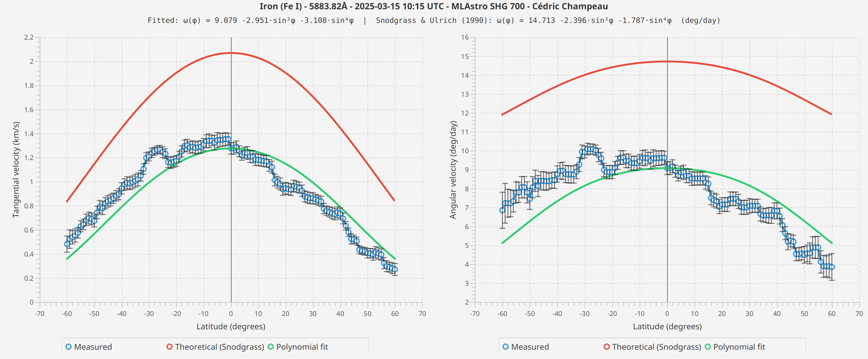
Fe I 5883 Å
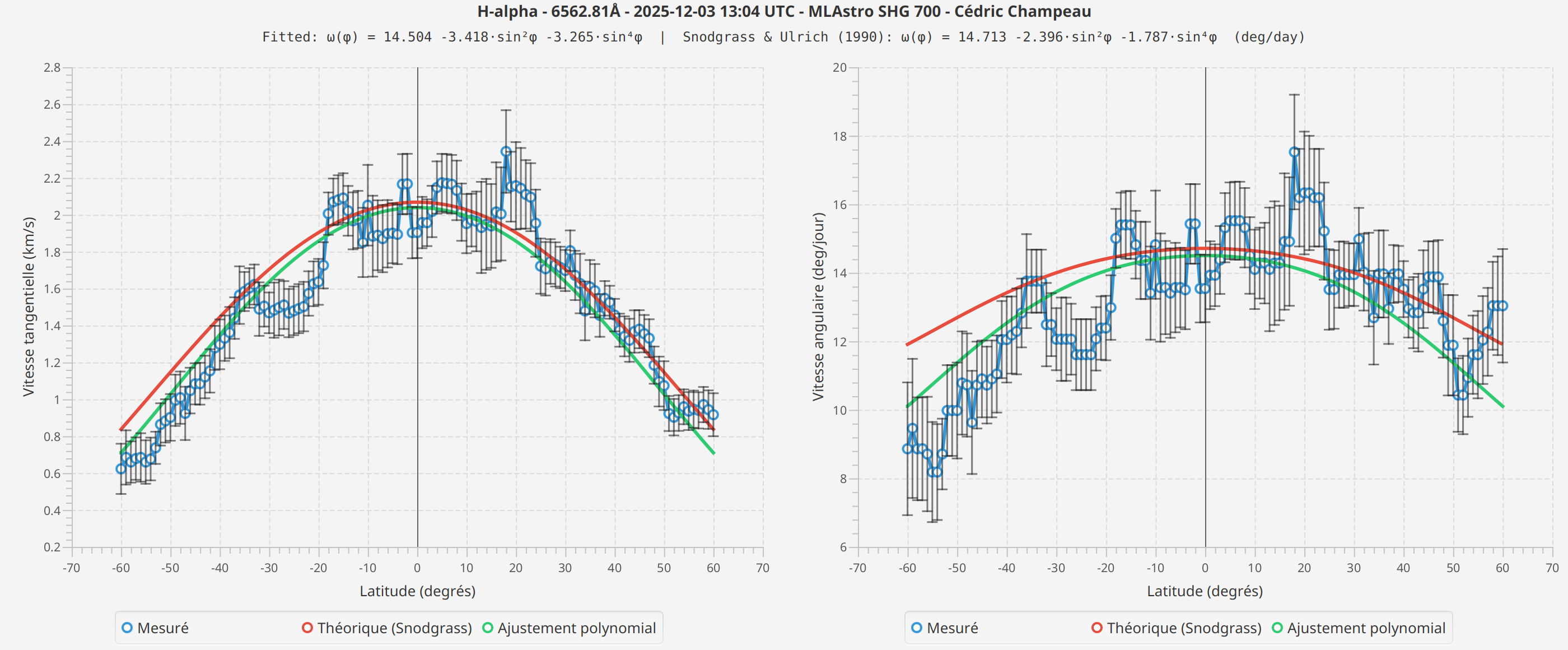
H-alpha
Observations
The measured profiles show the expected general shape: higher velocities at the equator, decreasing toward the poles. The fitted curves follow the theoretical Snodgrass profile reasonably well.
However, I observe differences between spectral lines that I cannot fully explain. The Fe I measurements show different absolute velocities than H-alpha, and the fitted coefficients differ between scans.
Several factors could contribute to these differences:
-
Formation height: Different spectral lines form at different heights in the solar atmosphere, and rotation rates may vary with height (as suggested by recent research from the CHASE mission)
-
Seeing conditions: The scans were taken on different dates with different atmospheric conditions
-
Line profile differences: H-alpha and Fe I have different line widths and depths, which may affect the Voigt fitting precision
-
Systematic effects: There may be instrumental or algorithmic factors I haven’t identified
I present these results as they are, without attempting to draw conclusions about which measurement is "correct" or what causes the observed differences. More measurements across different dates, spectral lines, and instruments would be needed to understand these variations.
Measuring in Practice
The quality of results depends heavily on atmospheric seeing. Poor seeing blurs the spectral lines and makes accurate center determination difficult. Best results are obtained with excellent seeing conditions and a well-focused instrument. Last but not least, a high spectral resolution is preferred, which is normally the case with Sol’Ex (HR) or the SHG 700.
You may also wonder which spectral line you should observe. I tested the algorithm with Fe I, Na D2 and H-alpha, giving the results below. In practice, strong absorption lines should in theory produce the best results, because:
-
The line depth should be sufficient for accurate fitting
-
The wings should be well-defined for Voigt fitting
-
The signal-to-noise ratio should be high
Very broad lines like Ca II K are too wide for accurate Voigt fitting and will produce unreliable results. Too narrow lines may also represent a challenge for Voigt fitting but may work too.
The Impact of the Spectral Line Detection
One subtle but important factor affecting the absolute accuracy of the measurements is the polynomial correction used during image reconstruction. Understanding this is essential for interpreting your results correctly.
During spectroheliograph processing, JSol’Ex computes a polynomial that maps each column position along the slit to the expected row position of the spectral line center. This polynomial is computed from the average of SER frames in the scan (a heuristic is used to include frames containing actual solar data, not sky background).
Such a detection is crucial because the spectral line is not straight across the slit due to optical phenomenons: it consistutes what we often call the "smile". Therefore, the line center might be at row 300 at column 500, but at row 350 at column 1000. The polynomial captures this curvature.
By measuring line positions relative to the polynomial, we effectively remove the optical distortion from our measurements. Without this reference, we would be measuring the sum of optical curvature plus Doppler shift, making it impossible to extract the tiny velocity signals we’re after.
A key question is: why can’t we just measure the absolute position of the spectral line in each frame and compute velocities directly?
The answer lies in the precision required. A velocity of 2 km/s corresponds to a wavelength shift of only ~0.04 Å at H-alpha. With a typical spectral dispersion of 0.1-0.2 Å/pixel, this is a shift of only 0.2 to 0.4 pixels.
The optical curvature across the slit, on the other hand, can easily span 10-30 pixels or more. Any attempt to measure absolute line positions would be completely dominated by this curvature, making Doppler detection impossible.
The polynomial serves as our reference baseline. By measuring how the line position in each individual frame deviates from the polynomial, we isolate the Doppler component from the optical component. This is the key insight that makes sub-pixel precision measurements possible, alongside the Voigt fitting.
A Word About Doppler Images
This, by the way, is also a reason why the Doppler images look different when scanning in RA vs DEC. Because this is a question that is often asked, and that it took months for me to understand the reason, I think it’s worth spending a bit of time explaining the phenomenon. I owe this explanation to Jean-François Pittet and Christian Buil, from a discussion weeks ago on the Sol’Ex mailing list.
RA Scanning vs DEC Scanning: A Critical Difference for Doppler Images
Spectroheliographs can scan the Sun in two directions:
-
RA scanning (Right Ascension): The slit is oriented North-South, and the scan proceeds East-West
-
DEC scanning (Declination): The slit is oriented East-West, and the scan proceeds North-South
This choice has profound implications for Doppler visibility, as explained by Jean-François Pittet on the Sol’Ex mailing list.
RA Scanning: Doppler Visible in Images
In RA scanning mode, each frame captures a vertical slice of the Sun from North pole to South pole. Over the course of the scan:
-
Early frames capture the East limb (approaching, blueshifted)
-
Middle frames capture the disk center (no radial velocity)
-
Late frames capture the West limb (receding, redshifted)
When JSol’Ex computes the polynomial from the average of all frames, the East and West contributions balance out. The blueshift from the East limb is canceled by the redshift from the West limb. The resulting polynomial represents the "neutral" baseline: approximately the line position at disk center with no Doppler shift.
As a result, when we reconstruct the image at pixel shift 0, the Doppler shifts become visible as contrast differences:
-
East limb appears darker (line shifted into the passband)
-
West limb appears brighter (line shifted out of the passband)
This is why Doppler images from RA scans show the characteristic East-West asymmetry.
DEC Scanning: Doppler "Absorbed" by the Polynomial
In DEC scanning mode, each frame captures a horizontal slice of the Sun from East to West. Here’s the critical difference: all pixels within a single frame see approximately the same Doppler shift.
For example, if the current frame is capturing the Eastern half of the disk:
-
All points in that frame are approaching us
-
All points have similar blueshift
When JSol’Ex computes the polynomial from the average of all frames, it doesn’t just capture the optical curvature: it also captures the average Doppler shift across the scan. But here’s the problem: the Doppler shift varies systematically across the scan (East frames are blueshifted, West frames are redshifted).
The polynomial effectively "absorbs" a weighted average of these Doppler shifts. When we then measure line positions relative to this polynomial, much of the Doppler signal has already been subtracted out. The resulting Doppler images will no longer show the rotation of the sun (which can also be a benefit, for other kind of observations).
This is why experienced spectroheliographers often prefer RA scanning for Doppler work: the Doppler signal is more visible and easier to detect.
The P-Angle Complication
There’s an additional subtlety: the Sun’s rotation axis is not perpendicular to the ecliptic. The P-angle (position angle of the rotation axis) varies throughout the year from about -26° to +26°.
Only twice per year (around early June and early December) is the P-angle close to zero. At these times:
-
RA scanning is truly parallel to the solar equator
-
The East-West Doppler pattern aligns perfectly with the scan direction
At other times, when P is non-zero:
-
The rotation axis is tilted relative to the scan direction
-
The Doppler pattern is rotated relative to the image axes
-
Some Doppler signal "leaks" into the polynomial average even in RA mode
This is one reason why differential rotation measurements can show slightly different results at different times of year, despite us taking the P and B0 angles into account.
Implications for Differential Rotation Measurements
This explains why RA scanning is essential for differential velocity measurements:
In RA mode, East and West limb points at the same latitude correspond to the same column on the slit (same slit position, different frames).
The polynomial value at that column is computed from the average of all frames (East limb, disk center, and West limb) so the Doppler shifts cancel out in the average.
When we compute (West - polynomial) - (East - polynomial), the polynomial terms are identical and cancel, leaving us with the true Doppler difference West - East.
In DEC mode, East and West limb points at the same latitude correspond to opposite ends of the slit (different columns, same frame). The polynomial at the East column is computed from frames that all see the East limb at that position, so the polynomial absorbs the blueshift. Similarly, the polynomial at the West column absorbs the redshift. When we compute the difference, these absorbed Doppler shifts don’t cancel: they subtract from our measurement, significantly reducing the measured signal.
This is why, in practice, DEC scans do not produce usable Doppler images or reliable differential velocity measurements.
Configuration Tips
-
Limb longitude (default 75°): Measurements closer to the limb give stronger Doppler signals but risk limb darkening effects
-
Latitude step (default 2°): Smaller values give finer resolution but longer processing times
-
Smoothing window: Should be at least 2× the latitude step for effective smoothing
Conclusion
Measuring differential rotation with amateur equipment would have seemed impossible just a few years ago. Pioneers like Peter Zetner or Christian Buil showed us the path. What I’m trying to do, as always with JSol’Ex, is to make this accessible to even more people at the cost of "magic", which is that some people will very likely share results without understanding the science behind it. I’m not too concerned by this, as I, myself, have been going this way: enjoying SHG image reconstruction, then figuring out how it works, then asking myself questions like "why is it even possible that we measure Doppler velocities so small?": this is an intellectual construct that takes time and we can do better, I think, at brining this to the masses, sharing our insights.
This feature joins the growing list of scientific capabilities in JSol’Ex: Ellerman bomb detection, active region identification, and now differential rotation measurement. Each of these brings professional-level analysis within reach of amateur astronomers, but, as always, be cautious with what I’m saying: I’m not a scientist, just an engineer. I have no doubts that I made approximations, or took liberties that I should probably not have taken.
However, I do think that this brings value to the ecosystem.
Bibliography
Scientific Papers
-
Howard, R. & Harvey, J. (1970) - Spectroscopic determinations of solar rotation. Sol Phys 12, 23-51
-
Snodgrass, H.B. (1984) - Separation of large-scale photospheric Doppler patterns. Sol Phys 94, 13-31
-
Beck, J.G. (2000) - A comparison of differential rotation measurements. Sol Phys 191, 47-70
-
Corbard, T. et al. (2025) - Rotational radial shear in the low solar photosphere. A&A 702, A93
